Custom presentation of trading history and creation of report diagrams
Andrey Azatskiy | 19 September, 2018
Introduction
One of the important aspects in financial trading is the ability to monitor performance and analyze your trading history. Past data allow you to track the trading dynamics and evaluate the overall performance of the strategy used. This is useful for all traders: for those, who perform operations manually and for algorithmic traders. In this article, I suggest creating tools that implement such a function.
The core piece of any trading activity is the trading algorithm which forms the Profit/Loss curve. Such an algorithm can be compared with a synthetic asset, the value of which is formed relative to the underlying asset (i.e. the traded instrument). For example, in options trading the Black-Scholes model formula is used for calculating such a synthetic asset based on the underlying asset price. But there is no such formula for a trading algorithm. Accordingly, launch of an algorithm can be compared to a long position of a synthetic symbol, the PL curve of which is formed by the algorithm's programmed logic. Profit formed by this "asset" can be unstable in different time periods. Even if it can be evaluated by some econometric model, this model cannot be unified. But how to track this asset and our trading stages? One of the suitable solutions is to monitor the algorithm trading retrospective and detect deviations from expected results.
I will not give advice on how to analyze algorithms, but will only provide a set of methods, which allow the presentation of the complete picture of your trading history. Based on data obtained, you will be able to build complex econometric models, calculate probability characteristics and make various conclusions.
This article will be divided into 2 sections. In the first (technical) section, I will describe methods for generating trading reports based on the bulk of information, which is stored in your terminals. This section deals with the source data used for analysis. In the second section, we will deal with the main values, by which we will evaluate the trading retrospective on the selected data. Data sampling can be varied: all assets or a selected symbol, for the entire available history or for a certain period of time. The analysis results will be presented in a separate file and briefly visualized in the terminal.
I used data from my real trading history for the analysis examples. Code implementation examples were prepared using a testing period, which I intentionally accumulated by trading on a demo account.
Chapter 1. Preparing data for the trade statistics analysis
Any analytics begins with the preparation of the source data. Here we deal with the trading history for a given period of time. The MetaTrader 5 terminal stores detailed reports. But sometimes too excessive information with a lot of details can hinder rather than help. In this section, we will try to create a readable, brief and informative sample of the trading history, which can further be processed and analyzed.
Trading history in MetaTrader 5 and related processing methods
Usually, a large number of records are made when unloading the trading history. Each position consists of entry/exit deals, which in turn can be performed in several stages. Also, there are situations of gradual position scaling and re-buys. In addition, the history has special lines for "alleged deals". Such deals may include:
- position opening/closure during variation margin related operations (FORTS);
- possible corrections of existing positions;
- depositing and withdrawal operations.
The inconvenience of reports is also connected with the fact that the history is sorted by the deal opening time. Deals may have different lifetime, therefore the display order of information related to actual position closure can be distorted. For example, the first deal is opened on June 1 and is closed on June 5. The second one is opened on June 2, and is closed on the same day. We fix the profit/loss of this deal earlier than of the first one, but in the table it will be later, because it was later opened.
Accordingly, the trading history recorded in this format is not appropriate for trading analysis. However, it reflects the entire history of operations on the analyzed account. MQL5 features a useful set of tools for working with the described data array. We will use this tool to present the data in a readable form. First, we need to arrange all the data as a trading history, sorted by traded assets and deals. For this purpose, let us create the following structures:
//+------------------------------------------------------------------+
//| Data structure of one selected deal                              |
//+------------------------------------------------------------------+
struct DealData
  {
   long              ticket;            // Ticket of the deal
   long              order;             // The number of the order opening the deal
   datetime          DT;                // Position open date
   long              DT_msc;            // Position open date in milliseconds
   ENUM_DEAL_TYPE    type;              // Open position type
   ENUM_DEAL_ENTRY   entry;             // Position entry type
   long              magic;             // The unique number of the position
   ENUM_DEAL_REASON  reason;            // How the order was placed
   long              ID;                // Position ID
   double            volume;            // Position volume (lots)
   double            price;             // Position entry price
   double            comission;         // Commission paid
   double            swap;              // Swap
   double            profit;            // Profit/loss
   string            symbol;            // Symbol
   string            comment;           // Comment specified at opening
   string            ID_external;       // External ID
  };
//+------------------------------------------------------------------+
//| Structure, which stores all deals of a certain position,         |
//| selected by ID                                                   |
//+------------------------------------------------------------------+
struct DealKeeper
  {
   DealData          deals[];           /* The list of all deals for this position (or several positions in case of position reversal)*/
   string            symbol;            // Symbol
   long              ID;                // ID of the position(s)
   datetime          DT_min;            // Opening date
   datetime          DT_max;            // Closing date
  };
You can see from the code, that the DealData structure contains an excessive description of deal parameters.
Our main structure will be DealKeeper. It contains the description of the position and all deals it includes. The main filter of a position in the terminal is its ID, which stays unchanged for all deals within the position. Therefore, if a position is reversed, the ID will be preserved, but the direction will be changed to opposite, that is why the DealKeeper structure will contain two positions. Filling of DealKeeper in our code is filtered based on the position ID.
Let's consider in detail how the structure is filled. It is done by the CDealHistoryGetter class, and namely its getHistory function:
//+-----------------------------------------------------------------------+
//| Class that extracts trading history from the terminal and             |
//| converts it to an easy-to-analyze view                                |
//+-----------------------------------------------------------------------+
class CDealHistoryGetter
  {
public:
   bool              getHistory(DealKeeper &deals[],datetime from,datetime till);                // returns data on all historic deals
   bool              getIDArr(ID_struct &ID_arr[],datetime from,datetime till);                  // returns a unique array of deal IDs
   bool              getDealsDetales(DealDetales &ans[],datetime from,datetime till);            // returns an array of deals, in which each line represents one specific deal
private:

   void              addArray(ID_struct &Arr[],const ID_struct &value);                          // add to the dynamic array
   void              addArray(DealKeeper &Arr[],const DealKeeper &value);                        // add to the dynamic array
   void              addArray(DealData &Arr[],const DealData &value);                            // add to the dynamic array
   void              addArr(DealDetales &Arr[],DealDetales &value);                              // add to the dynamic array
   void              addArr(double &Arr[],double value);                                         // add to the dynamic array

/*
    If there are InOut exits, inputParam will have more than one position.
    If there are no InOut exits, inputParam will only have one position!
*/
   void              getDeals_forSelectedKeeper(DealKeeper &inputParam,DealDetales &ans[]);      // forming a single entry based on a selected position for all positions in inputParam
   double            MA_price(double &prices[],double &lots[]);                                  // calculating the weighted average open price
   bool              isBorderPoint(DealData &data,BorderPointType &type);                        // get information whether this is a boundary point and the type of the point
   ENUM_DAY_OF_WEEK  getDay(datetime DT);                                                        // get the day from the date
   double            calcContracts(double &Arr[],GetContractType type);                          // get information on the last position volume
  };
Let's consider its implementation:
//+------------------------------------------------------------------+
//| Returns all data on historic deals                               |
//+------------------------------------------------------------------+
bool CDealHistoryGetter::getHistory(DealKeeper &deals[],datetime from,datetime till)
  {
   ArrayFree(deals);                                     // clear the results array
   ID_struct ID_arr[];
   if(getIDArr(ID_arr,from,till))                        // get unique IDs
     {
      int total=ArraySize(ID_arr);
      for(int i=0;i<total;i++)                           // loop through ID
        {
         DealKeeper keeper;                              // Keeper of a position's deals
         keeper.ID=ID_arr[i].ID;
         keeper.symbol=ID_arr[i].Symb;
         keeper.DT_max = LONG_MIN;
         keeper.DT_min = LONG_MAX;
         if(HistorySelectByPosition(ID_arr[i].ID))       // select all deals with the specified ID
           {
First, we need to get unique ID of the positions. For this purpose, we go through deal IDs in a continuous loop and form a structure with two fields: Symbol and Position ID. The obtained data will be required for the operation of the getHistory function.
The MQL5 language has a very useful function HistorySelectByPosition, which selects the entire history of deals with the passed ID. It will help us remove from the list unnecessary operations (account processing, deposit and withdrawal operations, etc.). As a result, a formed history of all changes of the position which occurred while it was open is recorded to memory. Data are sorted by date and time. We only need to use the HistoryDealsTotal function, which returns the total number of previously written deals with the specified ID.
int total_2=HistoryDealsTotal();
            for(int n=0;n<total_2;n++)                        // Loop through selected deals
              {
               long ticket=(long)HistoryDealGetTicket(n);
               DealData data;
               data.ID=keeper.ID;
               data.symbol=keeper.symbol;
               data.ticket= ticket;

               data.DT=(datetime)HistoryDealGetInteger(ticket,DEAL_TIME);
               keeper.DT_max=MathMax(keeper.DT_max,data.DT);
               keeper.DT_min=MathMin(keeper.DT_min,data.DT);
               data.order= HistoryDealGetInteger(ticket,DEAL_ORDER);
               data.type = (ENUM_DEAL_TYPE)HistoryDealGetInteger(ticket,DEAL_TYPE);
               data.DT_msc=HistoryDealGetInteger(ticket,DEAL_TIME_MSC);
               data.entry = (ENUM_DEAL_ENTRY)HistoryDealGetInteger(ticket,DEAL_ENTRY);
               data.magic = HistoryDealGetInteger(ticket,DEAL_MAGIC);
               data.reason= (ENUM_DEAL_REASON)HistoryDealGetInteger(ticket,DEAL_REASON);
               data.volume= HistoryDealGetDouble(ticket,DEAL_VOLUME);
               data.price = HistoryDealGetDouble(ticket,DEAL_PRICE);
               data.comission=HistoryDealGetDouble(ticket,DEAL_COMMISSION);
               data.swap=HistoryDealGetDouble(ticket,DEAL_SWAP);
               data.profit=HistoryDealGetDouble(ticket,DEAL_PROFIT);
               data.comment=HistoryDealGetString(ticket,DEAL_COMMENT);
               data.ID_external=HistoryDealGetString(ticket,DEAL_EXTERNAL_ID);

               addArray(keeper.deals,data);                  // Adding deals
              }

            if(ArraySize(keeper.deals)>0)
               addArray(deals,keeper);                       // Adding the position
           }
        }
      return ArraySize(deals) > 0;
     }
   else
      return false;                                          // If there are no unique IDs
  }
Thus, by going through each unique ID, we form an array of data describing the position. The DealKeeper array of structures reflects a detailed trading history of the current account, for the requested time period.
Preparing data for the analysis
In the previous section, we obtained data. Let us export the data to a file. Below is the list of deals for one of the analyzed positions:
| Ticket | Order | DT | DT msc | Type | Entry | Magic | Reason | ID | Volume | Price | Comission | Swap | Profit | Symbol | Comment | ID external |
|---|---|---|---|---|---|---|---|---|---|---|---|---|---|---|---|---|
| 10761601 | 69352663 | 23.11.2017 17:41 | 1,51146E+12 | DEAL_TYPE_BUY | DEAL_ENTRY_IN | 506789 | DEAL_REASON_EXPERT | 69352663 | 1 | 58736 | -0,5 | 0 | 0 | Si-12.17 | Open test position | 23818051 |
| 10761602 | 69352663 | 23.11.2017 17:41 | 1,51146E+12 | DEAL_TYPE_BUY | DEAL_ENTRY_IN | 506789 | DEAL_REASON_EXPERT | 69352663 | 1 | 58737 | -0,5 | 0 | 0 | Si-12.17 | Open test position | 23818052 |
| 10766760 | 0 | 24.11.2017 13:00 | 1,51153E+12 | DEAL_TYPE_SELL | DEAL_ENTRY_OUT | 0 | DEAL_REASON_VMARGIN | 69352663 | 2 | 58682 | 0 | 0 | -109 | Si-12.17 | [variation margin close] | |
| 10766761 | 0 | 24.11.2017 13:00 | 1,51153E+12 | DEAL_TYPE_BUY | DEAL_ENTRY_IN | 0 | DEAL_REASON_VMARGIN | 69352663 | 2 | 58682 | 0 | 0 | 0 | Si-12.17 | [variation margin open] | |
| 10769881 | 0 | 24.11.2017 15:48 | 1,51154E+12 | DEAL_TYPE_SELL | DEAL_ENTRY_OUT | 0 | DEAL_REASON_VMARGIN | 69352663 | 2 | 58649 | 0 | 0 | -66 | Si-12.17 | [variation margin close] | |
| 10769882 | 0 | 24.11.2017 15:48 | 1,51154E+12 | DEAL_TYPE_BUY | DEAL_ENTRY_IN | 0 | DEAL_REASON_VMARGIN | 69352663 | 2 | 58649 | 0 | 0 | 0 | Si-12.17 | [variation margin open] | |
| 10777315 | 0 | 27.11.2017 13:00 | 1,51179E+12 | DEAL_TYPE_SELL | DEAL_ENTRY_OUT | 0 | DEAL_REASON_VMARGIN | 69352663 | 2 | 58420 | 0 | 0 | -458 | Si-12.17 | [variation margin close] | |
| 10777316 | 0 | 27.11.2017 13:00 | 1,51179E+12 | DEAL_TYPE_BUY | DEAL_ENTRY_IN | 0 | DEAL_REASON_VMARGIN | 69352663 | 2 | 58420 | 0 | 0 | 0 | Si-12.17 | [variation margin open] | |
| 10780552 | 0 | 27.11.2017 15:48 | 1,5118E+12 | DEAL_TYPE_SELL | DEAL_ENTRY_OUT | 0 | DEAL_REASON_VMARGIN | 69352663 | 2 | 58417 | 0 | 0 | -6 | Si-12.17 | [variation margin close] | |
| 10780553 | 0 | 27.11.2017 15:48 | 1,5118E+12 | DEAL_TYPE_BUY | DEAL_ENTRY_IN | 0 | DEAL_REASON_VMARGIN | 69352663 | 2 | 58417 | 0 | 0 | 0 | Si-12.17 | [variation margin open] | |
| 10790453 | 0 | 28.11.2017 13:00 | 1,51187E+12 | DEAL_TYPE_SELL | DEAL_ENTRY_OUT | 0 | DEAL_REASON_VMARGIN | 69352663 | 2 | 58589 | 0 | 0 | 344 | Si-12.17 | [variation margin close] | |
| 10790454 | 0 | 28.11.2017 13:00 | 1,51187E+12 | DEAL_TYPE_BUY | DEAL_ENTRY_IN | 0 | DEAL_REASON_VMARGIN | 69352663 | 2 | 58589 | 0 | 0 | 0 | Si-12.17 | [variation margin open] | |
| 10793477 | 0 | 28.11.2017 15:48 | 1,51188E+12 | DEAL_TYPE_SELL | DEAL_ENTRY_OUT | 0 | DEAL_REASON_VMARGIN | 69352663 | 2 | 58525 | 0 | 0 | -128 | Si-12.17 | [variation margin close] | |
| 10793478 | 0 | 28.11.2017 15:48 | 1,51188E+12 | DEAL_TYPE_BUY | DEAL_ENTRY_IN | 0 | DEAL_REASON_VMARGIN | 69352663 | 2 | 58525 | 0 | 0 | 0 | Si-12.17 | [variation margin open] | |
| 10801186 | 0 | 29.11.2017 13:00 | 1,51196E+12 | DEAL_TYPE_SELL | DEAL_ENTRY_OUT | 0 | DEAL_REASON_VMARGIN | 69352663 | 2 | 58515 | 0 | 0 | -20 | Si-12.17 | [variation margin close] | |
| 10801187 | 0 | 29.11.2017 13:00 | 1,51196E+12 | DEAL_TYPE_BUY | DEAL_ENTRY_IN | 0 | DEAL_REASON_VMARGIN | 69352663 | 2 | 58515 | 0 | 0 | 0 | Si-12.17 | [variation margin open] | |
| 10804587 | 0 | 29.11.2017 15:48 | 1,51197E+12 | DEAL_TYPE_SELL | DEAL_ENTRY_OUT | 0 | DEAL_REASON_VMARGIN | 69352663 | 2 | 58531 | 0 | 0 | 32 | Si-12.17 | [variation margin close] | |
| 10804588 | 0 | 29.11.2017 15:48 | 1,51197E+12 | DEAL_TYPE_BUY | DEAL_ENTRY_IN | 0 | DEAL_REASON_VMARGIN | 69352663 | 2 | 58531 | 0 | 0 | 0 | Si-12.17 | [variation margin open] | |
| 10813418 | 0 | 30.11.2017 13:00 | 1,51205E+12 | DEAL_TYPE_SELL | DEAL_ENTRY_OUT | 0 | DEAL_REASON_VMARGIN | 69352663 | 2 | 58843 | 0 | 0 | 624 | Si-12.17 | [variation margin close] | |
| 10813419 | 0 | 30.11.2017 13:00 | 1,51205E+12 | DEAL_TYPE_BUY | DEAL_ENTRY_IN | 0 | DEAL_REASON_VMARGIN | 69352663 | 2 | 58843 | 0 | 0 | 0 | Si-12.17 | [variation margin open] | |
| 10816400 | 0 | 30.11.2017 15:48 | 1,51206E+12 | DEAL_TYPE_SELL | DEAL_ENTRY_OUT | 0 | DEAL_REASON_VMARGIN | 69352663 | 2 | 58609 | 0 | 0 | -468 | Si-12.17 | [variation margin close] | |
| 10816401 | 0 | 30.11.2017 15:48 | 1,51206E+12 | DEAL_TYPE_BUY | DEAL_ENTRY_IN | 0 | DEAL_REASON_VMARGIN | 69352663 | 2 | 58609 | 0 | 0 | 0 | Si-12.17 | [variation margin open] | |
| 10824628 | 0 | 01.12.2017 13:00 | 1,51213E+12 | DEAL_TYPE_SELL | DEAL_ENTRY_OUT | 0 | DEAL_REASON_VMARGIN | 69352663 | 2 | 58864 | 0 | 0 | 510 | Si-12.17 | [variation margin close] | |
| 10824629 | 0 | 01.12.2017 13:00 | 1,51213E+12 | DEAL_TYPE_BUY | DEAL_ENTRY_IN | 0 | DEAL_REASON_VMARGIN | 69352663 | 2 | 58864 | 0 | 0 | 0 | Si-12.17 | [variation margin open] | |
| 10828227 | 0 | 01.12.2017 15:48 | 1,51214E+12 | DEAL_TYPE_SELL | DEAL_ENTRY_OUT | 0 | DEAL_REASON_VMARGIN | 69352663 | 2 | 58822 | 0 | 0 | -84 | Si-12.17 | [variation margin close] | |
| 10828228 | 0 | 01.12.2017 15:48 | 1,51214E+12 | DEAL_TYPE_BUY | DEAL_ENTRY_IN | 0 | DEAL_REASON_VMARGIN | 69352663 | 2 | 58822 | 0 | 0 | 0 | Si-12.17 | [variation margin open] | |
| 10838074 | 0 | 04.12.2017 13:00 | 1,51239E+12 | DEAL_TYPE_SELL | DEAL_ENTRY_OUT | 0 | DEAL_REASON_VMARGIN | 69352663 | 2 | 59093 | 0 | 0 | 542 | Si-12.17 | [variation margin close] | |
| 10838075 | 0 | 04.12.2017 13:00 | 1,51239E+12 | DEAL_TYPE_BUY | DEAL_ENTRY_IN | 0 | DEAL_REASON_VMARGIN | 69352663 | 2 | 59093 | 0 | 0 | 0 | Si-12.17 | [variation margin open] | |
| 10840722 | 0 | 04.12.2017 15:48 | 1,5124E+12 | DEAL_TYPE_SELL | DEAL_ENTRY_OUT | 0 | DEAL_REASON_VMARGIN | 69352663 | 2 | 59036 | 0 | 0 | -114 | Si-12.17 | [variation margin close] | |
| 10840723 | 0 | 04.12.2017 15:48 | 1,5124E+12 | DEAL_TYPE_BUY | DEAL_ENTRY_IN | 0 | DEAL_REASON_VMARGIN | 69352663 | 2 | 59036 | 0 | 0 | 0 | Si-12.17 | [variation margin open] | |
| 10848185 | 0 | 05.12.2017 13:00 | 1,51248E+12 | DEAL_TYPE_SELL | DEAL_ENTRY_OUT | 0 | DEAL_REASON_VMARGIN | 69352663 | 2 | 58793 | 0 | 0 | -486 | Si-12.17 | [variation margin close] | |
| 10848186 | 0 | 05.12.2017 13:00 | 1,51248E+12 | DEAL_TYPE_BUY | DEAL_ENTRY_IN | 0 | DEAL_REASON_VMARGIN | 69352663 | 2 | 58793 | 0 | 0 | 0 | Si-12.17 | [variation margin open] | |
| 10850473 | 0 | 05.12.2017 15:48 | 1,51249E+12 | DEAL_TYPE_SELL | DEAL_ENTRY_OUT | 0 | DEAL_REASON_VMARGIN | 69352663 | 2 | 58881 | 0 | 0 | 176 | Si-12.17 | [variation margin close] | |
| 10850474 | 0 | 05.12.2017 15:48 | 1,51249E+12 | DEAL_TYPE_BUY | DEAL_ENTRY_IN | 0 | DEAL_REASON_VMARGIN | 69352663 | 2 | 58881 | 0 | 0 | 0 | Si-12.17 | [variation margin open] | |
| 10857862 | 0 | 06.12.2017 13:00 | 1,51257E+12 | DEAL_TYPE_SELL | DEAL_ENTRY_OUT | 0 | DEAL_REASON_VMARGIN | 69352663 | 2 | 59181 | 0 | 0 | 600 | Si-12.17 | [variation margin close] | |
| 10857863 | 0 | 06.12.2017 13:00 | 1,51257E+12 | DEAL_TYPE_BUY | DEAL_ENTRY_IN | 0 | DEAL_REASON_VMARGIN | 69352663 | 2 | 59181 | 0 | 0 | 0 | Si-12.17 | [variation margin open] | |
| 10860776 | 0 | 06.12.2017 15:48 | 1,51258E+12 | DEAL_TYPE_SELL | DEAL_ENTRY_OUT | 0 | DEAL_REASON_VMARGIN | 69352663 | 2 | 59246 | 0 | 0 | 130 | Si-12.17 | [variation margin close] | |
| 10860777 | 0 | 06.12.2017 15:48 | 1,51258E+12 | DEAL_TYPE_BUY | DEAL_ENTRY_IN | 0 | DEAL_REASON_VMARGIN | 69352663 | 2 | 59246 | 0 | 0 | 0 | Si-12.17 | [variation margin open] | |
| 10869047 | 0 | 07.12.2017 13:00 | 1,51265E+12 | DEAL_TYPE_SELL | DEAL_ENTRY_OUT | 0 | DEAL_REASON_VMARGIN | 69352663 | 2 | 59325 | 0 | 0 | 158 | Si-12.17 | [variation margin close] | |
| 10869048 | 0 | 07.12.2017 13:00 | 1,51265E+12 | DEAL_TYPE_BUY | DEAL_ENTRY_IN | 0 | DEAL_REASON_VMARGIN | 69352663 | 2 | 59325 | 0 | 0 | 0 | Si-12.17 | [variation margin open] | |
| 10871856 | 0 | 07.12.2017 15:48 | 1,51266E+12 | DEAL_TYPE_SELL | DEAL_ENTRY_OUT | 0 | DEAL_REASON_VMARGIN | 69352663 | 2 | 59365 | 0 | 0 | 80 | Si-12.17 | [variation margin close] | |
| 10871857 | 0 | 07.12.2017 15:48 | 1,51266E+12 | DEAL_TYPE_BUY | DEAL_ENTRY_IN | 0 | DEAL_REASON_VMARGIN | 69352663 | 2 | 59365 | 0 | 0 | 0 | Si-12.17 | [variation margin open] | |
| 10879894 | 0 | 08.12.2017 13:01 | 1,51274E+12 | DEAL_TYPE_SELL | DEAL_ENTRY_OUT | 0 | DEAL_REASON_VMARGIN | 69352663 | 2 | 59460 | 0 | 0 | 190 | Si-12.17 | [variation margin close] | |
| 10879895 | 0 | 08.12.2017 13:01 | 1,51274E+12 | DEAL_TYPE_BUY | DEAL_ENTRY_IN | 0 | DEAL_REASON_VMARGIN | 69352663 | 2 | 59460 | 0 | 0 | 0 | Si-12.17 | [variation margin open] | |
| 10882283 | 0 | 08.12.2017 15:48 | 1,51275E+12 | DEAL_TYPE_SELL | DEAL_ENTRY_OUT | 0 | DEAL_REASON_VMARGIN | 69352663 | 2 | 59421 | 0 | 0 | -78 | Si-12.17 | [variation margin close] | |
| 10882284 | 0 | 08.12.2017 15:48 | 1,51275E+12 | DEAL_TYPE_BUY | DEAL_ENTRY_IN | 0 | DEAL_REASON_VMARGIN | 69352663 | 2 | 59421 | 0 | 0 | 0 | Si-12.17 | [variation margin open] | |
| 10888014 | 0 | 11.12.2017 13:00 | 1,513E+12 | DEAL_TYPE_SELL | DEAL_ENTRY_OUT | 0 | DEAL_REASON_VMARGIN | 69352663 | 2 | 59318 | 0 | 0 | -206 | Si-12.17 | [variation margin close] | |
| 10888015 | 0 | 11.12.2017 13:00 | 1,513E+12 | DEAL_TYPE_BUY | DEAL_ENTRY_IN | 0 | DEAL_REASON_VMARGIN | 69352663 | 2 | 59318 | 0 | 0 | 0 | Si-12.17 | [variation margin open] | |
| 10890195 | 0 | 11.12.2017 15:48 | 1,51301E+12 | DEAL_TYPE_SELL | DEAL_ENTRY_OUT | 0 | DEAL_REASON_VMARGIN | 69352663 | 2 | 59280 | 0 | 0 | -76 | Si-12.17 | [variation margin close] | |
| 10890196 | 0 | 11.12.2017 15:48 | 1,51301E+12 | DEAL_TYPE_BUY | DEAL_ENTRY_IN | 0 | DEAL_REASON_VMARGIN | 69352663 | 2 | 59280 | 0 | 0 | 0 | Si-12.17 | [variation margin open] | |
| 10895808 | 0 | 12.12.2017 13:00 | 1,51308E+12 | DEAL_TYPE_SELL | DEAL_ENTRY_OUT | 0 | DEAL_REASON_VMARGIN | 69352663 | 2 | 58920 | 0 | 0 | -720 | Si-12.17 | [variation margin close] | |
| 10895809 | 0 | 12.12.2017 13:00 | 1,51308E+12 | DEAL_TYPE_BUY | DEAL_ENTRY_IN | 0 | DEAL_REASON_VMARGIN | 69352663 | 2 | 58920 | 0 | 0 | 0 | Si-12.17 | [variation margin open] | |
| 10897839 | 0 | 12.12.2017 15:48 | 1,51309E+12 | DEAL_TYPE_SELL | DEAL_ENTRY_OUT | 0 | DEAL_REASON_VMARGIN | 69352663 | 2 | 58909 | 0 | 0 | -22 | Si-12.17 | [variation margin close] | |
| 10897840 | 0 | 12.12.2017 15:48 | 1,51309E+12 | DEAL_TYPE_BUY | DEAL_ENTRY_IN | 0 | DEAL_REASON_VMARGIN | 69352663 | 2 | 58909 | 0 | 0 | 0 | Si-12.17 | [variation margin open] | |
| 10903172 | 0 | 13.12.2017 13:00 | 1,51317E+12 | DEAL_TYPE_SELL | DEAL_ENTRY_OUT | 0 | DEAL_REASON_VMARGIN | 69352663 | 2 | 59213 | 0 | 0 | 608 | Si-12.17 | [variation margin close] | |
| 10903173 | 0 | 13.12.2017 13:00 | 1,51317E+12 | DEAL_TYPE_BUY | DEAL_ENTRY_IN | 0 | DEAL_REASON_VMARGIN | 69352663 | 2 | 59213 | 0 | 0 | 0 | Si-12.17 | [variation margin open] | |
| 10905906 | 0 | 13.12.2017 15:48 | 1,51318E+12 | DEAL_TYPE_SELL | DEAL_ENTRY_OUT | 0 | DEAL_REASON_VMARGIN | 69352663 | 2 | 59072 | 0 | 0 | -282 | Si-12.17 | [variation margin close] | |
| 10905907 | 0 | 13.12.2017 15:48 | 1,51318E+12 | DEAL_TYPE_BUY | DEAL_ENTRY_IN | 0 | DEAL_REASON_VMARGIN | 69352663 | 2 | 59072 | 0 | 0 | 0 | Si-12.17 | [variation margin open] | |
| 10911277 | 0 | 14.12.2017 13:00 | 1,51326E+12 | DEAL_TYPE_SELL | DEAL_ENTRY_OUT | 0 | DEAL_REASON_VMARGIN | 69352663 | 2 | 58674 | 0 | 0 | -796 | Si-12.17 | [variation margin close] | |
| 10911278 | 0 | 14.12.2017 13:00 | 1,51326E+12 | DEAL_TYPE_BUY | DEAL_ENTRY_IN | 0 | DEAL_REASON_VMARGIN | 69352663 | 2 | 58674 | 0 | 0 | 0 | Si-12.17 | [variation margin open] | |
| 10912285 | 71645351 | 14.12.2017 14:48 | 1,51326E+12 | DEAL_TYPE_SELL | DEAL_ENTRY_OUT | 506789 | DEAL_REASON_EXPERT | 69352663 | 1 | 58661 | -0,5 | 0 | -13 | Si-12.17 | PartialClose position_2 | 25588426 |
| 10913632 | 0 | 14.12.2017 15:48 | 1,51327E+12 | DEAL_TYPE_SELL | DEAL_ENTRY_OUT | 0 | DEAL_REASON_VMARGIN | 69352663 | 1 | 58783 | 0 | 0 | 109 | Si-12.17 | [variation margin close] | |
| 10913633 | 0 | 14.12.2017 15:48 | 1,51327E+12 | DEAL_TYPE_BUY | DEAL_ENTRY_IN | 0 | DEAL_REASON_VMARGIN | 69352663 | 1 | 58783 | 0 | 0 | 0 | Si-12.17 | [variation margin open] | |
| 10919412 | 0 | 15.12.2017 13:00 | 1,51334E+12 | DEAL_TYPE_SELL | DEAL_ENTRY_OUT | 0 | DEAL_REASON_VMARGIN | 69352663 | 1 | 58912 | 0 | 0 | 129 | Si-12.17 | [variation margin close] | |
| 10919413 | 0 | 15.12.2017 13:00 | 1,51334E+12 | DEAL_TYPE_BUY | DEAL_ENTRY_IN | 0 | DEAL_REASON_VMARGIN | 69352663 | 1 | 58912 | 0 | 0 | 0 | Si-12.17 | [variation margin open] | |
| 10921766 | 0 | 15.12.2017 15:48 | 1,51335E+12 | DEAL_TYPE_SELL | DEAL_ENTRY_OUT | 0 | DEAL_REASON_VMARGIN | 69352663 | 1 | 58946 | 0 | 0 | 34 | Si-12.17 | [variation margin close] | |
| 10921767 | 0 | 15.12.2017 15:48 | 1,51335E+12 | DEAL_TYPE_BUY | DEAL_ENTRY_IN | 0 | DEAL_REASON_VMARGIN | 69352663 | 1 | 58946 | 0 | 0 | 0 | Si-12.17 | [variation margin open] | |
| 10927382 | 0 | 18.12.2017 13:00 | 1,5136E+12 | DEAL_TYPE_SELL | DEAL_ENTRY_OUT | 0 | DEAL_REASON_VMARGIN | 69352663 | 1 | 58630 | 0 | 0 | -316 | Si-12.17 | [variation margin close] | |
| 10927383 | 0 | 18.12.2017 13:00 | 1,5136E+12 | DEAL_TYPE_BUY | DEAL_ENTRY_IN | 0 | DEAL_REASON_VMARGIN | 69352663 | 1 | 58630 | 0 | 0 | 0 | Si-12.17 | [variation margin open] | |
| 10929913 | 0 | 18.12.2017 15:48 | 1,51361E+12 | DEAL_TYPE_SELL | DEAL_ENTRY_OUT | 0 | DEAL_REASON_VMARGIN | 69352663 | 1 | 58664 | 0 | 0 | 34 | Si-12.17 | [variation margin close] | |
| 10929914 | 0 | 18.12.2017 15:48 | 1,51361E+12 | DEAL_TYPE_BUY | DEAL_ENTRY_IN | 0 | DEAL_REASON_VMARGIN | 69352663 | 1 | 58664 | 0 | 0 | 0 | Si-12.17 | [variation margin open] | |
| 10934874 | 0 | 19.12.2017 13:00 | 1,51369E+12 | DEAL_TYPE_SELL | DEAL_ENTRY_OUT | 0 | DEAL_REASON_VMARGIN | 69352663 | 1 | 58635 | 0 | 0 | -29 | Si-12.17 | [variation margin close] | |
| 10934875 | 0 | 19.12.2017 13:00 | 1,51369E+12 | DEAL_TYPE_BUY | DEAL_ENTRY_IN | 0 | DEAL_REASON_VMARGIN | 69352663 | 1 | 58635 | 0 | 0 | 0 | Si-12.17 | [variation margin open] | |
| 10936988 | 0 | 19.12.2017 15:48 | 1,5137E+12 | DEAL_TYPE_SELL | DEAL_ENTRY_OUT | 0 | DEAL_REASON_VMARGIN | 69352663 | 1 | 58629 | 0 | 0 | -6 | Si-12.17 | [variation margin close] | |
| 10936989 | 0 | 19.12.2017 15:48 | 1,5137E+12 | DEAL_TYPE_BUY | DEAL_ENTRY_IN | 0 | DEAL_REASON_VMARGIN | 69352663 | 1 | 58629 | 0 | 0 | 0 | Si-12.17 | [variation margin open] | |
| 10941561 | 0 | 20.12.2017 13:00 | 1,51377E+12 | DEAL_TYPE_SELL | DEAL_ENTRY_OUT | 0 | DEAL_REASON_VMARGIN | 69352663 | 1 | 58657 | 0 | 0 | 28 | Si-12.17 | [variation margin close] | |
| 10941562 | 0 | 20.12.2017 13:00 | 1,51377E+12 | DEAL_TYPE_BUY | DEAL_ENTRY_IN | 0 | DEAL_REASON_VMARGIN | 69352663 | 1 | 58657 | 0 | 0 | 0 | Si-12.17 | [variation margin open] | |
| 10943405 | 0 | 20.12.2017 15:48 | 1,51378E+12 | DEAL_TYPE_SELL | DEAL_ENTRY_OUT | 0 | DEAL_REASON_VMARGIN | 69352663 | 1 | 58684 | 0 | 0 | 27 | Si-12.17 | [variation margin close] | |
| 10943406 | 0 | 20.12.2017 15:48 | 1,51378E+12 | DEAL_TYPE_BUY | DEAL_ENTRY_IN | 0 | DEAL_REASON_VMARGIN | 69352663 | 1 | 58684 | 0 | 0 | 0 | Si-12.17 | [variation margin open] | |
| 10948277 | 0 | 21.12.2017 13:00 | 1,51386E+12 | DEAL_TYPE_SELL | DEAL_ENTRY_OUT | 0 | DEAL_REASON_VMARGIN | 69352663 | 1 | 58560 | 0 | 0 | -124 | Si-12.17 | [variation margin close] | |
| 10948278 | 0 | 21.12.2017 13:00 | 1,51386E+12 | DEAL_TYPE_BUY | DEAL_ENTRY_IN | 0 | DEAL_REASON_VMARGIN | 69352663 | 1 | 58560 | 0 | 0 | 0 | Si-12.17 | [variation margin open] | |
| 10949780 | 0 | 21.12.2017 15:45 | 1,51387E+12 | DEAL_TYPE_SELL | DEAL_ENTRY_OUT | 0 | DEAL_REASON_CLIENT | 69352663 | 1 | 58560 | 0 | 0 | 0 | Si-12.17 | [instrument expiration] | 26163141 |
The used example is based on the history of USDRUR Futures deals performed on a demo account, in the FORTS market. From the table, we can see that the position entry was split into two orders with an equal lot. Exit was also performed in two deals. The IDs of the orders which opened deals for each entry and exit (except for the variation margin) were non-zero. But the last deal that closed the position, originated from an order with a zero ID. This happened because the position was not closed manually, but it was closed because of the asset expiration.
This is a visually represented history, which reflects deals (including the so called "alleged" orders) executed within one position. However, it is still inconvenient for the final position analysis and requires further improvements. We need a table with each line reflecting the financial result of a position and providing related information.
Let's create the following structure:
//+------------------------------------------------------------------+
//| Structure, which stores the financial result and                 |
//| main information about the selected position                     |
//+------------------------------------------------------------------+
struct DealDetales
  {
   string            symbol;                // Symbol
   datetime          DT_open;               // Open date
   ENUM_DAY_OF_WEEK  day_open;              // Day of the week of position opening
   datetime          DT_close;              // Close date
   ENUM_DAY_OF_WEEK  day_close;             // Day of the week of position closing
   double            volume;                // Volume (lots)
   bool              isLong;                // Sign of Long/Short
   double            price_in;              // Position entry price
   double            price_out;             // Position exit price
   double            pl_oneLot;             // Profit/loss if one lot were traded
   double            pl_forDeal;            // Real profit/loss obtained, taking into account the commission
   string            open_comment;          // Comment at the time of opening
   string            close_comment;         // Comment at the time of closing
  };
The structure is formed by the getDealsDetales method. It uses three key private methods:
- isBorderPoint, which determines if this is a "border" position (if it is set by the trader and if it closes/opens the position);
- MA_price, which calculates the actual position opening/closing price;
- calcContracts, which calculates the number of contracts in the market at the time of position existence.
Let us view in detail the MA_price method. For example, if the open position involved several contracts at different prices, it would be incorrect to use the price of the very first deal as the position opening price. This will produce errors in further calculations. We will use a weighted average value. We will average position Open/Close prices and weight them by the volume of opened deals. This is how the logic is implemented in a code:
//+------------------------------------------------------------------+
//| Calculating the weighted average open price                      |
//+------------------------------------------------------------------+
double CDealHistoryGetter::MA_price(double &prices[],double &lots[])
  {
   double summ=0;                           // The sum of weighted prices
   double delemetr=0;                       // The sum of weights
   int total=ArraySize(prices);
   for(int i=0;i<total;i++)                 // Summation loop
     {
      summ+=(prices[i]*lots[i]);
      delemetr+=lots[i];
     }
   return summ/delemetr;                    // Calculating the average
  }
As for traded lots: this is a more complicated case, but it is not difficult to understand. Let's consider an example of dynamic position management: we gradually add or reduce the number of lots:
| In | Out | |
|---|---|---|
| Open (t1) | 1 | 0 |
| t2 | 2 | 0 |
| t3 | 5 | 3 |
| t4 | 1 | 0 |
| t5 | 0 | 1 |
| t6 | 1 | 0 |
| t7 | 0 | 1 |
| t8 | 1 | 0 |
| t9 | 0 | 1 |
| Close (t10) | 0 | 5 |
| Total | 11 | 11 |
During the position lifetime, we additionally bought and sold the traded asset multiple times (sometimes in turns, and sometimes almost simultaneously). Thus, we had 11 buy and sell lots. But this does not mean that the maximum reached position volume was equal to 11 lots. Let's write down all entries and exits: position increase and entries will have the sign +, exist and position decrease will have the sign -. We will calculate the sum similarly to the PL curve.
| Deal volume | Position volume | |
|---|---|---|
| deal 1 | 1 | 1 |
| deal 2 | 2 | 3 |
| deal 3 | 5 | 8 |
| deal 4 | -3 | 5 |
| deal 5 | 1 | 6 |
| deal 6 | -1 | 5 |
| deal 7 | 1 | 6 |
| deal 8 | -1 | 5 |
| deal 9 | 1 | 6 |
| deal 10 | -1 | 5 |
| deal 11 | -5 | 0 |
It can be seen from this table, that the maximum reached volume was 8 lots. This is the required value.
Here is the code of the function reflecting the number of lots:
//+------------------------------------------------------------------+
//| Calculating the real volume of the position and                  |
//| obtaining information about the volume of the last position      |
//+------------------------------------------------------------------+
double CDealHistoryGetter::calcContracts(double &Arr[],GetContractType type)
  {
   int total;

   if((total=ArraySize(Arr))>1)                        // if the array size is greater than one
     {
      double lotArr[];
      addArr(lotArr,Arr[0]);                           // adding the first lot to the array
      for(int i=1;i<total;i++)                         // loop from the second array element
         addArr(lotArr,(lotArr[i-1]+Arr[i]));          // adding the sum of the previous and the current lot to the array (lotArr[i-1]+Arr[i]))

      if(type==GET_REAL_CONTRACT)
         return lotArr[ArrayMaximum(lotArr)];          // return the actual maximum traded lot
      else
         return lotArr[ArraySize(lotArr)-1];           // return the last traded lot
     }
   else
      return Arr[0];
  }
In addition to the simple counting of lots, the function shows the last active lot (equal to 5 in our example).
Let's consider the isBorderPoint function, which was created for filtering unnecessary deals. Based on the data structure, we can determine the importance of a deal using 4 variables:
- Order ID;
- ENUM_DEAL_ENTRY — entry, exit, reversal;
- ENUM_DEAL_TYPE — buying/selling;
- ENUM_DEAL_REASON — order placing method.
Creating the enumeration:
//+--------------------------------------------------------------------+
//| Auxiliary enumeration showing the type of a particular record      |
//| The record is represented by the DealData structure                |
//+--------------------------------------------------------------------+
enum BorderPointType
  {
   UsualInput,          // usual entry type (DEAL_ENTRY_IN) - the beginning of a deal
   UsualOutput,         // usual exit type (DEAL_ENTRY_OUT) - the end of the deal
   OtherPoint,          // balance operation, position correction, withdrawals, variation margin — to be ignored
   InOut,               // position reversal (DEAL_ENTRY_INOUT)
   OutBy                // a position closed by an opposite order (DEAL_ENTRY_OUT_BY)
  };
We need four of the five variants presented above. All the deals to be ignored are gathered in OtherPoint. The combinations of parameters for each of the enumeration variants are presented in the table. The function code is available in the files attached below.
| Enumeration variant | Order ID | ENUM_DEAL_ENTRY | ENUM_DEAL_TYPE | ENUM_DEAL_REASON |
|---|---|---|---|---|
| UsualInput | >0 | DEAL_ENTRY_IN | DEAL_TYPE_BUY | DEAL_REASON_CLIENT |
| DEAL_REASON_EXPERT | ||||
| DEAL_TYPE_SELL | DEAL_REASON_WEB | |||
| DEAL_REASON_MOBILE | ||||
| UsualOut | >=0(=0 if closed by expiration) | DEAL_ENTRY_OUT | DEAL_TYPE_BUY | DEAL_REASON_CLIENT |
| DEAL_REASON_EXPERT | ||||
| DEAL_REASON_WEB | ||||
| DEAL_TYPE_SELL | DEAL_REASON_MOBILE | |||
| DEAL_REASON_SL | ||||
| DEAL_REASON_TP | ||||
| DEAL_REASON_SO | ||||
| OtherPoint | 0 | DEAL_ENTRY_IN | DEAL_TYPE_BUY | DEAL_REASON_ROLLOVER |
| DEAL_TYPE_SELL | ||||
| DEAL_TYPE_BALANCE | ||||
| DEAL_TYPE_CREDIT | ||||
| DEAL_TYPE_CHARGE | ||||
| DEAL_TYPE_CORRECTION | ||||
| DEAL_TYPE_BONUS | DEAL_REASON_VMARGIN | |||
| DEAL_TYPE_COMMISSION | ||||
| DEAL_TYPE_COMMISSION_DAILY | ||||
| DEAL_ENTRY_OUT | DEAL_TYPE_COMMISSION_MONTHLY | |||
| DEAL_TYPE_COMMISSION_AGENT_DAILY | ||||
| DEAL_TYPE_COMMISSION_AGENT_MONTHLY | ||||
| DEAL_TYPE_INTEREST | DEAL_REASON_SPLIT | |||
| DEAL_TYPE_BUY_CANCELED | ||||
| DEAL_TYPE_SELL_CANCELED | ||||
| DEAL_DIVIDEND | ||||
| DEAL_DIVIDEND_FRANKED | ||||
| DEAL_TAX | ||||
| InOut | >0 | DEAL_ENTRY_INOUT | DEAL_TYPE_BUY | DEAL_REASON_CLIENT |
| DEAL_REASON_EXPERT | ||||
| DEAL_TYPE_SELL | DEAL_REASON_WEB | |||
| DEAL_REASON_MOBILE | ||||
| OutBy | >0 | DEAL_ENTRY_OUT_BY | DEAL_TYPE_BUY | DEAL_REASON_CLIENT |
| DEAL_REASON_EXPERT | ||||
| DEAL_TYPE_SELL | DEAL_REASON_WEB | |||
| DEAL_REASON_MOBILE |
We will form the required history using the getDeals_forSelectedKeeper method. Let's view its general logic, and then analyze in detail actions for each of the above described enumeration variants (starting from line 303).
//+------------------------------------------------------------------+
//| One record for each selected position is formed in в inputParam  |
//+------------------------------------------------------------------+

void CDealHistoryGetter::getDeals_forSelectedKeeper(DealKeeper &inputParam,DealDetales &ans[])
  {
   ArrayFree(ans);
   int total=ArraySize(inputParam.deals);
   DealDetales detales;                                          // the variable in which results from the following loop will be added
   detales.symbol=inputParam.symbol;
   detales.volume= 0;
   detales.pl_forDeal=0;
   detales.pl_oneLot=0;
   detales.close_comment= "";
   detales.open_comment = "";
   detales.DT_open=0;

// Flag indicating whether the position should be added to the set
   bool isAdd=false;
   bool firstPL_setted=false;
// Arrays of entry prices, exit prices, entry lots, exit lots, contracts
   double price_In[],price_Out[],lot_In[],lot_Out[],contracts[]; // line 404

   for(int i=0;i<total;i++)                                      // loop through deals (all deals have the same ID, but there can be more than one position if the deal type is InOut)
     {
      BorderPointType type;                                      // deal type, line 408
      double pl_total=0;

      if(isBorderPoint(inputParam.deals[i],type))                // find out if it is a border deal and the deal type, line 301
        {
          // line 413
        } // line 414
      else
        {
/*
         If it is not a border deal, simply record the financial result.
         There can only be variation margin and various correction operations.
         Deposit and withdrawal operation are filtered out when obtaining initial data
*/
         detales.pl_forDeal+=(inputParam.deals[i].profit+inputParam.deals[i].comission);
         detales.pl_oneLot+=inputParam.deals[i].profit/calcContracts(contracts,GET_LAST_CONTRACT);
        }
     }

// Filtering active positions and do not save them
   if(isAdd && PositionSelect(inputParam.symbol))                 // line 541
     {
      if(PositionGetInteger(POSITION_IDENTIFIER)==inputParam.ID)
         isAdd=false;
     }                                                            // line 546

// Save fixed and already inactive positions
   if(isAdd)
     {
      detales.price_in=MA_price(price_In,lot_In);
      detales.price_out=MA_price(price_Out,lot_Out);

      detales.volume=calcContracts(contracts,GET_REAL_CONTRACT);
      addArr(ans,detales);
     }
  }
Arrays are declared on the function's line 404. They will further be used under the condition specified in lines 411-414. Only border points are considered inside this condition, i.e. the deals that open/close or increase/partially close a position.
If the deal does not fall under the first condition, the only required action is to calculate its profit/loss. Our history contains actually obtained profit/loss, which is divided into deals. Each deal reflects a change in PL, starting from deal preceding the execution of the analyzed deal. The total position profit is equal to the sum of PLs of all these deals. If we calculate the profit/loss as a difference between open and close prices, the number of factors will be ignored, such as slippage, volume changes within a position, commission and fees.
On code lines 541-546, we filter open positions, which are not saved as a result. The following is calculated at the end of the function: the open and close prices as well as the maximum position volume which was in the market.
The type variable is used for filtering border points. If opening or deal increase is being performed at the moment, we switch to the next condition, which starts from line 413 (see the full text of the method in the attachment).
if(type==UsualInput)                                                   // if it is initial entry or position increase
  {
   if(detales.DT_open==0)                                              // assign position opening date
     {
      detales.DT_open=inputParam.deals[i].DT;
      detales.day_open=getDay(inputParam.deals[i].DT);
     }
   detales.isLong=inputParam.deals[i].type==DEAL_TYPE_BUY;             // determine the position direction
   addArr(price_In,inputParam.deals[i].price);                         // save the entry price
   addArr(lot_In,inputParam.deals[i].volume);                          // save the number of lots

   pl_total=(inputParam.deals[i].profit+inputParam.deals[i].comission);
   detales.pl_forDeal+=pl_total;                                       // the profit/loss of a deal taking into account the commission
   if(!firstPL_setted)
     {
      detales.pl_oneLot=pl_total/inputParam.deals[i].volume;           // the profit/loss of a deal taking into account the commission if trading one lot
      firstPL_setted=true;
     }
   else
      detales.pl_oneLot=inputParam.deals[i].profit/calcContracts(contracts,GET_LAST_CONTRACT);

   if(StringCompare(inputParam.deals[i].comment,"")!=0)                // comment to a deal
      detales.open_comment+=(StringCompare(detales.open_comment,"")==0 ?
                             inputParam.deals[i].comment :
                             (" | "+inputParam.deals[i].comment));
   addArr(contracts,inputParam.deals[i].volume);                       // adding volume of a deal with the "+" sign
  }
We also assign the position open date and calculate profit (total and per one lot). Position closure is performed under another condition:
if(type==UsualOut || type==OutBy)                         // Position closure
  {
/*
           We do not save the result right away, because there can be several exits
           Therefore leave the flag on to avoid data loss
*/
   if(!isAdd)isAdd=true;                                  // Flag to save the position

   detales.DT_close=inputParam.deals[i].DT;               // Closing date
   detales.day_close=getDay(inputParam.deals[i].DT);      // Closing date
   addArr(price_Out,inputParam.deals[i].price);           // Save the exit prices
   addArr(lot_Out,inputParam.deals[i].volume);            // Save the exit volume

   pl_total=(inputParam.deals[i].profit+inputParam.deals[i].comission);          // The profit/loss of a deal taking into account the commission
   detales.pl_forDeal+=pl_total;

   if(i==total-1)
      detales.pl_oneLot+=pl_total/calcContracts(contracts,GET_LAST_CONTRACT);    // The profit/loss of a deal taking into account the commission if trading one lot
   else
      detales.pl_oneLot+=inputParam.deals[i].profit/calcContracts(contracts,GET_LAST_CONTRACT); // The profit/loss of a deal taking into account the commission if trading one lot

   if(StringCompare(inputParam.deals[i].comment,"")!=0)                          // Deal comment
      detales.close_comment+=(StringCompare(detales.close_comment,"")==0 ?
                              inputParam.deals[i].comment :
                              (" | "+inputParam.deals[i].comment));
   addArr(contracts,-inputParam.deals[i].volume);                                // Adding volume of a deal with the "-" sign
  }
This condition assigns the position exit date and calculates the profit of a deal. There can be multiple entries and exits, so the conditions can occur several times.
The InOut condition is the combination of the second and first conditions. It only occurs once and results in a position reversal.
if(type==InOut)                                                                 // Position reversal
  {
/*
           Part 1:
           Save the previous position
*/
   firstPL_setted=true;
   double closingContract=calcContracts(contracts,GET_LAST_CONTRACT);           // Closed contract
   double myLot=inputParam.deals[i].volume-closingContract;                     // Opened contract

   addArr(contracts,-closingContract);                                          // Add the deal volume with the "-" sign
   detales.volume=calcContracts(contracts,GET_REAL_CONTRACT);                   // Get the maximum real deal volume which actually existed in the market

   detales.DT_close=inputParam.deals[i].DT;                                     // Closing date
   detales.day_close=getDay(inputParam.deals[i].DT);                            // Closing date
   addArr(price_Out,inputParam.deals[i].price);                                 // Exit price
   addArr(lot_Out,closingContract);                                             // Exit volume

   pl_total=(inputParam.deals[i].profit*closingContract)/inputParam.deals[i].volume;        // Calculating PL of the closing deal
   double commission_total=(inputParam.deals[i].comission*closingContract)/inputParam.deals[i].volume;
   detales.pl_forDeal+=(pl_total+commission_total);
   detales.pl_oneLot+=pl_total/closingContract;                                 // The profit/loss of a deal taking into account the commission if trading one lot
   if(StringCompare(inputParam.deals[i].comment,"")!=0)                         // Save the closing comment
      detales.open_comment+=(StringCompare(detales.open_comment,"")==0 ?
                             inputParam.deals[i].comment :
                             (" | "+inputParam.deals[i].comment));

   detales.price_in=MA_price(price_In,lot_In);                                  // Get the position entry price (average)
   detales.price_out=MA_price(price_Out,lot_Out);                               // Get the position exit price (average)
   addArr(ans,detales);                                                         // Add the formed position
   if(isAdd)isAdd=false;                                                        // Reset the flag if it was enabled

                                                                                // Clearing part of data
   ArrayFree(price_In);
   ArrayFree(price_Out);
   ArrayFree(lot_In);
   ArrayFree(lot_Out);
   ArrayFree(contracts);
   detales.close_comment="";
   detales.open_comment="";
   detales.volume=0;

/*
           Part 2:
           Save the new position after deleting part of data from the details array
*/

   addArr(contracts,myLot);                                                     // Add the position opening lot

   pl_total=((inputParam.deals[i].profit+inputParam.deals[i].comission)*myLot)/inputParam.deals[i].volume; // the profit/loss of a deal taking into account the commission
   detales.pl_forDeal=pl_total;
   detales.pl_oneLot=pl_total/myLot;                                            //T he profit/loss of a deal taking into account the commission if trading one lot
   addArr(lot_In,myLot);                                                        // Add the entry lot

   detales.open_comment=inputParam.deals[i].comment;                            // Save the comment

   detales.DT_open=inputParam.deals[i].DT;                                      // Save the opening date
   detales.day_open=getDay(inputParam.deals[i].DT);                             // Save the opening day
   detales.isLong=inputParam.deals[i].type==DEAL_TYPE_BUY;                      // Determine the deal direction
   addArr(price_In,inputParam.deals[i].price);                                  // Save the entry price
  }
The result of the above calculations is a table, each line of which reflects the main parameters of a position. Now, we can produce all the required calculations based on positions, and not deals which the positions consist of.
| Instrument | Open DT | Open day | Close DT | Close day | Contracts | Direction | Price open | Price close | PL for 1 lot | PL for position | Open comment | Close comment |
|---|---|---|---|---|---|---|---|---|---|---|---|---|
| RTS-12.17 | 17.11.2017 19:53 | FRIDAY | 17.11.2017 19:54 | FRIDAY | 2.00000000 | Long | 113200.00000000 | 113180.00000000 | -25.78000000 | -55.56000000 | ||
| RTS-12.17 | 17.11.2017 19:54 | FRIDAY | 17.11.2017 19:54 | FRIDAY | 2.00000000 | Short | 113175.00000000 | 113205.00000000 | -58.47000000 | -79.33000000 | ||
| RTS-12.17 | 17.11.2017 19:58 | FRIDAY | 17.11.2017 19:58 | FRIDAY | 1.00000000 | Short | 113240.00000000 | 113290.00000000 | -63.44000000 | -63.44000000 | ||
| RTS-12.17 | 17.11.2017 19:58 | FRIDAY | 17.11.2017 19:58 | FRIDAY | 1.00000000 | Long | 113290.00000000 | 113250.00000000 | -51.56000000 | -51.56000000 | ||
| Si-12.17 | 17.11.2017 20:00 | FRIDAY | 17.11.2017 20:00 | FRIDAY | 10.00000000 | Long | 59464.40000000 | 59452.80000000 | -23.86000000 | -126.00000000 | ||
| Si-12.17 | 17.11.2017 20:00 | FRIDAY | 17.11.2017 20:00 | FRIDAY | 5.00000000 | Short | 59453.20000000 | 59454.80000000 | -5.08666667 | -13.00000000 | ||
| Si-12.17 | 17.11.2017 20:02 | FRIDAY | 17.11.2017 20:02 | FRIDAY | 1.00000000 | Short | 59460.00000000 | 59468.00000000 | -9.00000000 | -9.00000000 | ||
| Si-12.17 | 17.11.2017 20:02 | FRIDAY | 17.11.2017 20:03 | FRIDAY | 2.00000000 | Long | 59469.00000000 | 59460.00000000 | -14.50000000 | -20.00000000 | ||
| Si-12.17 | 21.11.2017 20:50 | TUESDAY | 21.11.2017 21:06 | TUESDAY | 2.00000000 | Long | 59467.00000000 | 59455.00000000 | -13.00000000 | -26.00000000 | ||
| Si-12.17 | 23.11.2017 17:41 | THURSDAY | 21.12.2017 15:45 | THURSDAY | 2.00000000 | Long | 58736.50000000 | 58610.50000000 | -183.00000000 | -253.50000000 | Open test position | Open test position | PartialClose position_2 | [instrument expiration] |
| RTS-12.17 | 23.11.2017 18:07 | THURSDAY | 14.12.2017 14:45 | THURSDAY | 1.00000000 | Short | 115680.00000000 | 114110.00000000 | 1822.39000000 | 1822.39000000 | Open test position_2 | |
| RTS-3.18 | 30.01.2018 20:22 | TUESDAY | 30.01.2018 20:22 | TUESDAY | 2.00000000 | Short | 127675.00000000 | 127710.00000000 | -61.01000000 | -86.68000000 | ||
| RTS-3.18 | 30.01.2018 20:24 | TUESDAY | 30.01.2018 20:24 | TUESDAY | 1.00000000 | Long | 127730.00000000 | 127710.00000000 | -26.49000000 | -26.49000000 | ||
| RTS-3.18 | 30.01.2018 20:24 | TUESDAY | 30.01.2018 20:25 | TUESDAY | 1.00000000 | Long | 127730.00000000 | 127680.00000000 | -60.21000000 | -60.21000000 | ||
| RTS-3.18 | 30.01.2018 20:25 | TUESDAY | 30.01.2018 20:25 | TUESDAY | 1.00000000 | Long | 127690.00000000 | 127660.00000000 | -37.72000000 | -37.72000000 | ||
| RTS-3.18 | 30.01.2018 20:25 | TUESDAY | 30.01.2018 20:26 | TUESDAY | 1.00000000 | Long | 127670.00000000 | 127640.00000000 | -37.73000000 | -37.73000000 | ||
| RTS-3.18 | 30.01.2018 20:29 | TUESDAY | 30.01.2018 20:30 | TUESDAY | 1.00000000 | Long | 127600.00000000 | 127540.00000000 | -71.45000000 | -71.45000000 |
Chapter 2. Creating a custom trading report
Now, let's create a class, which will generate a trading report. First, we define the requirements for the report.
- The report will contain standard PL graphs and expanded ones for a more efficient evaluation of performance. The construction of charts starts from zero (regardless of the initial capital) - this will increase the objectivity of the evaluation.
- We will generate the "Buy and hold" chart of the strategy, which is similar to the PL graph (the both will be calculated by the same function). Both of these diagrams will be built on all assets which appear in the report.
- The main coefficients and trading results should be displayed in a table.
- Additional charts will be built, such as PL by days.
At the end, we will present the analyzed parameters in the form of variable charts and download all the calculation results to csv files. The examples given here are based on real history for a certain period of time. This history is attached below. The script for visualization and data downloading will contain the following functions: the first one will show examples on the attached trading history, and the second one will be based on your own history available in your terminal.
This part of the article will provide a minimum of code. Instead, we will focus on examining the data obtained and explaining their meaning. All parts of the class, which creates the report, are commented in detail, so you can easily understand them. For a better understanding of the described functions, I provide here the structure of the class.
class CReportGetter
  {
public:
                     CReportGetter(DealDetales &history[]);                      // Only history in the prepared format can be given
                     CReportGetter(DealDetales &history[],double balance);       // We can set here both history and balance relative to which calculations will be performed
                    ~CReportGetter();

   bool              get_PLChart(PL_chartData &pl[],
                                 PL_chartData &pl_forOneLot[],
                                 PL_chartData &Indicative_pl[],
                                 string &Symb[]);                                // PL graphs

   bool              get_BuyAndHold(PL_chartData &pl[],
                                    PL_chartData &pl_forOneLot[],
                                    PL_chartData &Indicative_pl[],
                                    string &Symb[]);                             // Buy and hold charts

   bool              get_PLHistogram(PL_chartData &pl[],
                                     PL_chartData &pl_forOneLot[],
                                     string &Symb[]);                            // Profit and loss accumulation histogram

   bool              get_PL_forDays(PLForDaysData &ans,
                                    DailyPL_calcBy calcBy,
                                    DailyPL_calcType type,
                                    string &Symb[]);                             // PL by days of the week

   bool              get_extremePoints(PL_And_Lose &total,
                                       PL_And_Lose &forDeal,
                                       string &Symb[]);                          // Extreme points (the highest and lowest values within a deal and with accumulation)

   bool              get_AbsolutePL(PL_And_Lose &total,
                                    PL_And_Lose &average,
                                    string &Symb[]);                             // Absolute values (accumulated and average PL)

   bool              get_PL_And_Lose_percents(PL_And_Lose &ans,string &Symb[]);  // The diagram of distribution of winning and losing deals

   bool              get_totalResults(TotalResult_struct &res,string &Symb[]);   // The table of the main variables

   bool              get_PLDetales(PL_detales &ans,string &Symb[]);              // A brief summary of the PL graph

   void              get_Symbols(string &SymbArr[]);                             // Getting the list of symbols available in the history

private:
   DealDetales       history[];                                                  // Stores the history of trades
   double            balance;                                                    // Stores the balance value

   void              addArray(DealDetales &Arr[],DealDetales &value);            // Adding data to the dynamic array
   void              addArray(PL_chartData &Arr[],PL_chartData &value);          // Adding data to the dynamic array
   void              addArray(string &Arr[],string value);                       // Adding data to the dynamic array
   void              addArray(datetime &Arr[],datetime value);                   // Adding data to the dynamic array

   void              sortHistory(DealDetales &arr[],bool byClose);               // Sorting history by open or close date

   void              cmpDay(int i,ENUM_DAY_OF_WEEK day,ENUM_DAY_OF_WEEK etaloneDay,PLDrowDown &ans);      // Filling the PLDrowDown structure

   bool              isSymb(string &Symb[],int i);                               // Check if the i-th symbol from the history is in the Symb array

   bool              get_PLChart_byHistory(PL_chartData &pl[],
                                           PL_chartData &pl_forOneLot[],
                                           PL_chartData &Indicative_pl[],
                                           DealDetales &historyData[]);          // PL graphs based on the passed history

   ENUM_DAY_OF_WEEK  getDay(datetime DT);                                        // Getting the trading date from the date

  };
3 types of PL diagrams
To create a profit and loss diagram, we sort the initial data by the position closing date. No explanation is needed here, since this is a standard chart. It will consist of two charts with position closing dates along the X axis. The first one is the actual PL graph, while the second one shows the accumulated drawdown relative to the maximum PL value, in percent. Let's consider 3 types of diagrams.
- The standard accumulated profit charts.
- Accumulated profit chart not taking into account the trading volume, as if we traded one lot on all of the symbols, throughout the entire history.
- The profit and loss chart, normalized to the maximum lost (or profitable) lot. If the PL chart is in the red zone, then divide the i-th loss by the maximum profitable lot. If the chart is in the green zone, then divide the i-th profit by the maximum loss lot.
The first two diagrams allow understanding how the change in the traded volume influences the profit/loss. The third one allows imagining an extreme situation: what would happen if a series of losses suddenly began, and these losses were equal to the maximum possible historical loss per lot (which is practically impossible). It shows how many maximum losses in a row the PL can have before it reaches 0 (all profits will be lost) - or vice versa, what would happen if all losses were covered by a series of maximum profits. These diagram types are shown below:
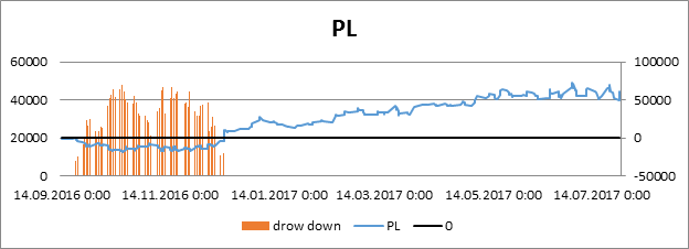
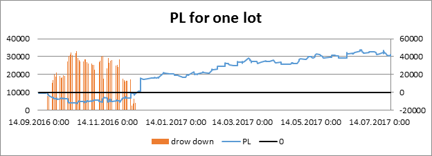
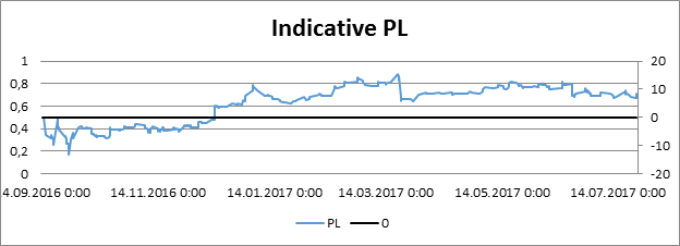
PL graph for 1-lot trading is more attractive than the real graph. Profit during real trading exceeded the hypothetical "one-lot" trading by as little as 30%. The lot size ranged from 1 to 10. Drawdown in percent reached 30,000%. The situation is not as terrible as it sounds. As mentioned above, the PL graph construction starts from zero, while the drawdown is calculated relative to the maximum value of the PL curve. At some moment, when the loss had not yet reached the maximum value (the red zone on the graph), the profit rose by several rubles, and then fell to -18,000 rubles. That is why the drawdown is so huge. The actual drawdown did not exceed 25% per one lot and 50 % on actual deals.


The normalized PL graph is stuck at one value. This indicates the need to change the trading approach (such as to change the lot management method) or to re-optimize trading algorithms. The PL graph with a variable lot looks worse than the one-lot graph for the same period, but such position management still had positive results: drawdown jumps became weaker.
The class, which generates the trading report, is called CReportGetter, and the diagrams are built by the get_PLChart_byHistory method. This method is provided with detailed comments in the source code files. It operates as follows:
- It iterates through the passed history.
- Each position is included in the calculation of PL, maximum profit and drawdown.
- Drawdown is calculated as an accumulated value relative to the maximum profit reached. If the PL graph immediately starts to drop into the red zone, the drawdown will be recalculated each time a new lowest value appears. In this case, the maximum profit is zero, and the drawdown on the i-th and all previous elements is recalculated relative to the maximum loss. Here drawdown is equal to 100%. Once the maximum profit rises above zero (the PL curve enters the positive part of the graph), then the drawdown will be further calculated only relative to the maximum profit.
Let us perform analysis by comparing three charts. This method allows detecting much more flaws, than the use of a single standard Profit and Loss diagram. PL graphs of the "buy and hold" strategy are built according to the same algorithm. I will provide only one of the graphs as an example. The other ones will be built automatically upon the visualization script launch.
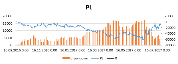
The figure shows that if we traded the same assets with the same volumes according to the "Buy and hold" strategy, the PL graph would hardly come to zero, and the drawdown would be about 80,000 rubles (instead of the 70,000 rubles of the maximum profit achieved).
PL accumulation chart
This chart represents two histograms, one over another. Their construction differs from the standard PL graph. The profit histogram is created by the gradual accumulation of only profitable trades. If the i-th position is losing, we ignore its value and write the previous value to the i-th time interval. The histogram of losing deals is built according to mirror logic. Below are the profit and loss histogram charts based on our data.
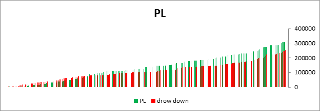
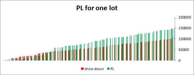
The usual PL graph is a simple difference between the profit and loss histograms. The first thing that catches the eye straight away is the great difference between the real obtained profit and the traded one. The real obtained profit exceeded one-lot trading by approximately 30%, while the histogram chart analysis showed a difference of almost 50%. The missing 20% of profit stem from the difference in the dynamics of profit growth over losses on the first and second graphs. Let us illustrate this analysis. We build two profit and loss dynamics charts based on these histograms. The formula is very simple:
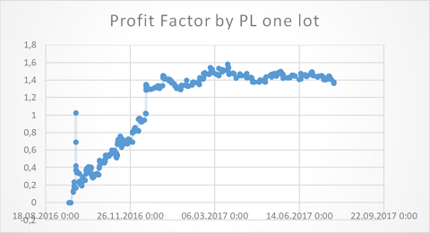
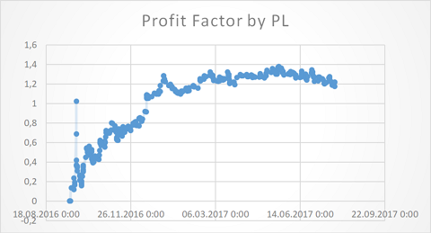
We see that the dynamics of profit was growing at the beginning, if compared to losses. This is an ideal development of events: with each new deal, the distance of the profit histogram from the histogram of losing deals increases. If the profit growth over loses has positive dynamics throughout the entire trading, we get one of the best results. Profits are accumulated more quickly, and losses are increased with the same or lower rate in relation to profits.
The next segment of the charts shows that the percentage difference between the profit and loss histograms stopped increasing, and continued to move in a sideways trend. If the sideways trend of growth of profits over losses has any interval above one, this is also seen as positive. If the interval is equal to one, then the PL curve will approach zero (each new profit will be equal to each new loss). If the sideways interval is below 1, we have started to lose our money. In other words, these diagrams visualize a gradual change in the profit factor. Here are the diagrams:
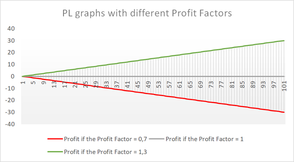
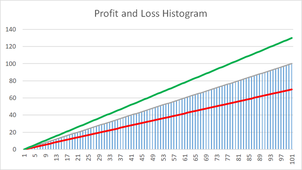
The blue histogram shows a linear accumulation of loss (the scale ranges from 0 to 100).
- Green: histogram of losses * 1.3,
- Gray: histogram of losses * 1,
- Red: histogram of losses * 0.7.
The charts show that the profit factor (the ratio showing excess of profits over losses) should always be greater than one. The ideal development is the gradual growth of the PF. The PL graph will grow exponentially in this case. Unfortunately, this is unrealistic in the long term, but such a situation can happen in a short lucky period, if you increase the lot after each profitable deal. Based on this example, we can assert with 100% confidence that the main point in trading is not how the PL graph changes, but how the histogram of profitable and losing deals behaves, and consequently, what the dynamics of the profit factor change is.
Now let's consider the 20% lost profits. See the diagram of one-lot profit growth dynamics: profit growth stopped in the interval [1.4 — 1.6]. This is higher than [1.2 - 1.4]. Over time, this difference covered 20% of potential profit. In other words, the position size management gave positive results. If you use methods such as martingale or anti-martingale, these charts, especially the metrics calculated on their basis, can provide a lot of useful information for analysis. These charts are built by the get_PLHistogram function.
Profit and loss by day
Anyone who has ever tested robots in the strategy Tester, already knows this diagram. The histogram meaning and construction methodology are the same. Additionally, I implemented the possibility to construct it using absolute values (obtained by simple summation of profits and losses by days) and averaged data. The simple averaging method is used in the attached class. Other averaging methods (mode/median, weighted averaging) can produce even more interesting results. You can implement these averaging types yourself.
Also, I added the total amount of deals (positive and negative): it shows the number of deals by days. A combined analysis of this histogram with the PL graph by day gives a more accurate trading picture in the context of a week. For example, it will enable the detection of situation when we have 50 small losses and 3 profits for a day, and these large profits cover all the losses. Here is an example of a bar chart built on absolute data and position closing price.
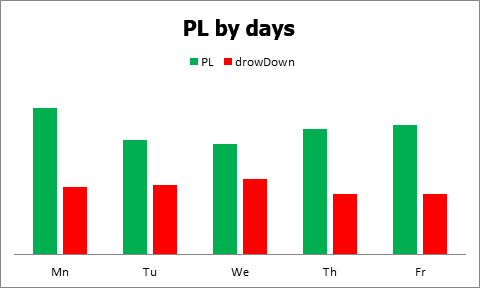
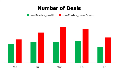
The diagram on all days of the week shows that positive deals covered losses, but the number of loss deals was always greater (generally, this situation is typical of the algorithmic trading). Also, the number of negative deals never increased the number of positive ones by more than 25%, which is also generally normal.
Extreme points and absolute values
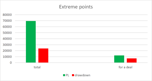
The diagram of extreme points is a histogram of 4 bars divided into two groups. The extreme points are the maximum and minimum deviations on the PL graph (the maximum achieved profit and the maximum accumulated drawdown). Two more bars show the maximum profitable and losing deal. Both groups are based on real trading data, not on profit and loss data per one deal. Calculation of the maximum profit on the PL curve is the highest point on the graph. The maximum drawdown calculation methodology was described above. Here is the relating formula:
This diagram illustrates the maximum spread of profit and loss. The share of maximum drawdown compared to the maximum profit was 30%. The value of the maximum losing deal compared to the most profitable one was 60%. In the code, this is implemented as a loop with a gradual comparison of the PL curve data according to the indicated conditions.
As for absolute values, they are best represented in a tabular form. These are also represented as two groups of data: the first one is the sum of all profits and the sum of all losses; the second group is the average profit and loss values within the analyzed history.
| Total | Average | |
|---|---|---|
| Profit | 323237 | 2244.701 |
| Drawdown | 261534 | 1210.806 |
Tables with a brief PL graph summary and the main trading results
These tables reflect numeric characteristics of trading performance. Table creation code contains the following structures:
//+------------------------------------------------------------------+
//| The structure of trading results                                 |
//+------------------------------------------------------------------+
struct TotalResult_struct
  {
   double            PL;                                // Total profit or loss
   double            PL_to_Balance;                     // Ratio of PL to current balance
   double            averagePL;                         // Average profit or loss
   double            averagePL_to_Balance;              // Ratio of averagePL to current balance
   double            profitFactor;                      // Profit factor
   double            reciveryFactor;                    // Recovery factor
   double            winCoef                            // Payoff factor
   double            dealsInARow_to_reducePLTo_zerro;/* If it's profit now, the number of deals in a row with the maximum loss per deal,
                                                        to bring current account Profit down to zero.
                                                        If it's loss  now, the number of deals in a row with the maximum profit per deal,
                                                        to cover losses down to zero*/

   double            maxDrowDown_byPL;                  // Maximum drawdown relative to PL
   double            maxDrowDown_forDeal;               // Maximum drawdown per deal
   double            maxDrowDown_inPercents;            // Maximum drawdown relative to PL as a percentage of the current balance
   datetime          maxDrowDown_byPL_DT;               // The date of the maximum drawdown relative to PL
   datetime          maxDrowDown_forDeal_DT             //The date of the maximum drawdown per deal

   double            maxProfit_byPL;                    // Maximum profit on PL
   double            maxProfit_forDeal;                 // Maximum profit per deal
   double            maxProfit_inPercents;              // Maximum profit on PL as a percentage of the current balance
   datetime          maxProfit_byPL_DT;                 // The date of the maximum profit on PL
   datetime          maxProfit_forDeal_DT;              // The date of the maximum profit per deal
  };
//+------------------------------------------------------------------+
//| Part of the PL_detales structure (declared below)                |
//+------------------------------------------------------------------+
struct PL_detales_item
  {
   int               orders;                            // Number of deals
   double            orders_in_Percent;                 // Number of orders as % to the total number of orders
   int               dealsInARow;                       // Deals in a row
   double            totalResult;                       // Total result in the deposit currency
   double            averageResult;                     // Average result in the deposit currency
  };
//+-------------------------------------------------------------------+
//| A brief PL graph summary divided into 2 main blocks               |
//+-------------------------------------------------------------------+
struct PL_detales
  {
   PL_detales_item   profits;                           // Information on profitable deals
   PL_detales_item   loses;                             // Information on losing deals
  };
The first structure, TotalResult_struct, is a summary of key values throughout the requested trading history. It includes the necessary values (profit and loss per trade, etc.), and the calculated trading performance coefficients.
The second and third structures are interrelated. PL_detales is the main structure containing a brief summary on the profit and loss histogram. The following results were obtained on the analyzed history:
| Value | Meaning |
|---|---|
| PL | 65039 |
| PL to balance | 21,8986532 |
| Average PL | 180,1634349 |
| Average PL to balance | 0,06066109 |
| Profit factor | 1,25097242 |
| Recovery factor | 3,0838154 |
| Payoff ratio | 1,87645863 |
| Deals till PL is brought down to zero | 24,16908213 |
| Drawdown relative to PL | -23683 |
| Drawdown per 1-lot deal | -2691 |
| Drawdown relative to the balance | -0,07974074 |
| Date of drawdown relative to PL | 24.07.2017 13:04 |
| Date of drawdown per 1-lot deal | 31.01.2017 21:53 |
| Profit on PL | 73034 |
| Profit per 1-lot deal | 11266 |
| Profit relative to the balance | 0,24590572 |
| date of profit on PL | 27.06.2017 23:42 |
| Date of profit per 1-lot deal | 14.12.2016 12:51 |
The second table is as follows:
| Profits | Losses | |
|---|---|---|
| Average result | 2244.701 | -1210,81 |
| Deals in a row | 5 | 10 |
| Total number of deals | 144 | 216 |
| Deals in % | 0,398892 | 0,598338 |
| Total result: | 323237 | -261534 |
The distribution of losing and profitable positions can be represented as a donut chart:
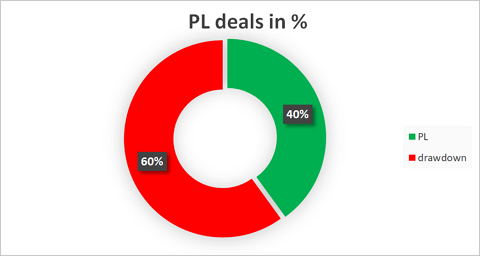
As can be seen from the result, 40% of deals were positive.
Conclusion
It's no secret that when using algorithms in trading, it is not enough just to optimize and launch them. The result of running an algorithm to the full capability immediately after optimization, without adjusting it to fit the portfolio structure, may bring rather unexpected results. Of course, traders often play Russian roulette. However, there are a lot of reasonable traders who prefer to think over their future steps. History analysis technique used in the article provides such traders an interesting opportunity, enabling them to test the optimality of chosen weights assigned to each trading algorithm.
One of the interesting application spheres is to analyze different portfolio calculation methods and to test them on the available trading history, and then to compare the new portfolio performance with the actual results. This can be done through one-lot trading, which is calculated based on the real trading history in the first chapter of this article. However, please note that the data obtained in such calculations will be approximate, because they do not take into account the asset liquidity, commissions and various force majors.
The following files are attached to the article:
- The CSV file dealHistory.csv containing the trading history (located in the folder MQL5\Files\article_4803) - examples provided in this article are based on this history.
- Source files for MetaTrader 5, which are located under MQL5\Scripts\Get_TradigHistory
- The test script project, divided into the parts described below
- File ListingFilesDirectory.mqh – a library of WinAPI functions, which allows to use files throughout the computer.
- Files Tests.mqh and Tests.mq5 save a report to a file after creating folders at the passed paths.
- File PlotCharts.mqh – draws report visualization charts in the terminal.
- The test script Get_TradingHistory.mq5 having two functions:
- The test_1 function accepts path to the attached testing history file as one parameter and path to the results tab as the second parameter. This function generates a report on the test files passed as the first function parameter.
- The second test_2 function accepts the second folder path (the paths must be different) as a parameter. A report on your trading will be saved in that folder.
Main files:
- DealHistoryGetter.mqh contains functions implementing data downloading methods described in the first chapter of the article.
- ReportGetter.mqh features an implementation of the trading report generation mechanism. The class contained in this file accepts the generated history and processes it.
