Application of the Eigen-Coordinates Method to Structural Analysis of Nonextensive Statistical Distributions
MetaQuotes | 8 August, 2012
Contents
- Introduction
- 1. Q-Gaussians in Econometrics
- 2. Eigen-Coordinates
- 3. Nonextensive Probability Distributions
- 4. If it looks like a cat... it might not be a cat
- Conclusion
- References
- Appendix. Analysis of SP500 daily returns with Q-Gaussian
Introduction
In 1988, Constantino Tsallis proposed the generalization of Boltzmann-Gibbs-Shannon statistical mechanics [1] where he presented a notion of nonextensive entropy.
An important consequence of the generalization of entropy appeared to be the existence of new distribution types [2] playing the key role in the new statistical mechanics (Q-Exponential and Q-Gaussian):
![]()
It was found that these distribution types can be used to describe a good deal of experimental data in systems with long-range memory, systems with long-range forces and strongly correlated systems.
The entropy is closely related to information [7]. The generalization of statistical mechanics based on information theory was presented in [8-9]. New nonextensive statistical mechanics has proved very useful for econometrics [10-17]. For example, the Q-Gaussian distribution well describes wide wings (tails) of distributions of increments of financial instrument quotes (q~1.5). That said, most distributions of increments of financial time series transform into normal distributions (q=1) at larger scales (months, years) [10].
It was naturally expected that such generalization of statistical mechanics would result in an analog of the central limit theorem for the q-Gaussian distributions. But this was shown to be wrong in [18] - the limit distribution of the sum of strongly correlated random variables is analytically different from q-Gaussians.
However, a problem of another kind appeared: it turned out that numerical values of the exact solution found were very close to the Q-Gaussian ("numerically similar, analytically different"). To analyze the differences between the functions and obtain the best parameters of the Q-Gaussian distribution a series expansion was used in [18]. The relationships of these functions led to power expansion in the q parameter characterizing the degree of system nonextensivity.
The major problem of applied statistics is the problem of accepting statistical hypotheses. It was long considered impossible to be solved [19-20] requiring a special tool (something like an electron microscope) which would allow to see more than what is possible using methods of modern applied statistics.
The eigen-coordinates method introduced in [21] enables us to reach a deeper level - the analysis of structural properties of functional relationships. This very fine method can be used to solve a variety of problems. Operator expansions of functions corresponding to the above nonextensive distributions were demonstrated in [22].
This article will deal with the eigen-coordinates method and examples of its practical use. It contains a lot of formulas which are of great importance towards understanding the essence of the method. After repeating all the calculations, you will be able to plot function expansions for functions of interest on your own.
1. Q-Gaussians in Econometrics
The Q-Gaussian distribution plays a very important role in econometrics [4,10-17].
To get a general understanding of the current research level, one can refer to the works of Dr. Claudio Antonini "q-Gaussians in Finance" [23] and "The Use of the q-Gaussian Distribution in Finance" [24].
Let us briefly outline the main results.
")
Fig. 1. Science methodology (Slide 4 "The Use of the q-Gaussian Distribution in Finance")
The main particulars of financial time series are set forth in Fig. 2:
")
Fig. 2. Properties of financial time series (Slide 3 "The Use of the q-Gaussian Distribution in Finance")
A lot of theoretical models that are used to describe financial time series lead to the Q-Gaussian distribution:
")
Fig. 3. Theoretical models and the Q-Gaussian (Slide 27 "The Use of the q-Gaussian Distribution in Finance")
The Q-Gaussian distribution is also used for phenomenological description of distributions of quotes:
")
Fig. 4. Sample analysis of the S&P 500 daily returns (Slide 8 "The Use of the q-Gaussian Distribution in Finance")
Working with real data poses a problem of function identification:
")
Fig. 5. The problem of distribution function identification (Slide 14 "q-Gaussians in Finance")
Both papers by Dr. Claudio Antonini stress the importance of correct identification of functions for building adequate models of physical processes:
")
Fig. 6. Conclusions drawn in "q-Gaussians in Finance" and "The Use of the q-Gaussian Distribution in Finance" (Dr. Claudio Antonini, 2010, 2011)
- q-Gaussian Stock Price Dynamics, (Michael English, 2008)
- q-Gaussian European Options (Michael English, 2008)
- q-Gaussian Random Deviates & Distribution, (Michael English, 2008)
- q-Gaussian Portfolios (Michael English, 2008)
- q-Gaussian Risk Measures (Michael English, 2008)
- Expected Value & Value at Risk for Lognormal Asset (Michael English, 2008)
2. Eigen-Coordinates
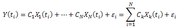
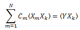
The eigen-coordinates expansion is as follows:
![]()
where C1…CN are constants and X1(t),..,XN(t) are the "eigen-coordinates".
Such linear expansions are very convenient and often used in data analysis. For example, an exponential function on a logarithmic scale turns into a straight line (its slope can easily be calculated using linear regression). Thus, there is no need for non-linear optimization (fitting) in order to determine the function parameters.
Logarithmic scale will however be of little help when dealing with more complex functions (e.g. the sum of two exponents) - the function will not appear as a straight line. And a non-linear optimization will be required to determine the function coefficients.
There are cases where experimental data can be equally well explained using several functions, all of which correspond to different models of physical processes. What function to choose? Which one will provide a more adequate picture of reality outside experimental data?
Correct function identification is vital for the analysis of complex systems (e.g. financial time series) - every distribution corresponds to a certain physical process and we will be able to better understand the dynamics and general properties of complex systems having chosen an adequate model.
Applied statistics [19, 20] states that there is no criterion which allows you to reject a wrong statistical hypothesis. The eigen-coordinates method throws a completely new light on this problem (hypothesis acceptance).
The function used for the description of experimental data can be viewed as a solution to a certain differential equation. Its form determines the structure of the eigen-coordinates expansion.
A peculiar feature of the eigen-coordinates expansion is that all data generated by the function Y(t) are linear in structure in the eigen-coordinates basis X1(t)..XN(t) of the function Y(t). Data generated by any other function F(t) will in this basis no longer appear as a straight line (they will look linear in the eigen-coordinates basis of the function F(t)).
This fact allows to accurately identify functions, thus greatly facilitating the work with statistical hypotheses.
2.1. The Eigen-Coordinates Method
The concept behind the method is to build the eigen-coordinates Xk(t) in the form of operators based on the function Y(t).
It can be done using mathematical analysis whereby the eigen-coordinates Xk(t) take on the form of integral convolutions and the expansion is determined by the structure of the differential equation which is satisfied by the function Y(t). Further, a problem of determining the coefficients C1.. CN crops up.
In the orthogonal basis expansion (e.g. when determining the Fourier transform coefficients), expansion coefficients are calculated by projecting the vector on the basis and the desired result is obtained due to the orthogonality of basis functions.
This is not suitable in our case as there is no information on the orthogonality of X1(t)… XN(t).
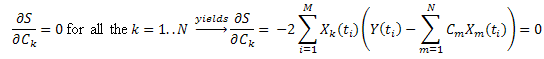
2.2. Calculation of Expansion Coefficients Using the Least Squares Method
The coefficients Ck can be calculated using the least squares method. This problem reduces to solving a system of linear equations.
Suppose that:
![]()
For virtually every measurement of ![]() there is an error
there is an error ![]() :
:
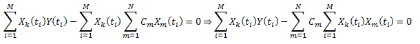
Minimize the sum of squared deviations:

Introducing the notation:  , it can be written as follows:
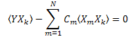
Thus, we get a system of linear equations in C1...CN (k=1..N):
The "correlation" matrix is symmetric: ![]() .
.
In some cases, the eigen-coordinates expansion may appear more convenient in integral form:
![]()
It allows to reduce the impact of errors (due to averaging) but requires additional calculations.
2.3. An Example of the R(x) Function Expansion
Let us have a look at the eigen-coordinates expansion of the following function:
![]()
This function generates several statistical distributions [21]:
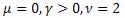 - the normal (Gaussian) distribution;
 - the Poisson distribution;
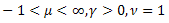 - the gamma distribution;
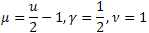 - the
- the  distribution;
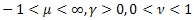 - Schtauffer's distribution which includes the Weibull distribution as a special case
  .
.
In addition, it is also well suited to describe relaxation processes:
 - the ordinary exponential function;
 - the stretched exponential function;
 - the power relaxation function.
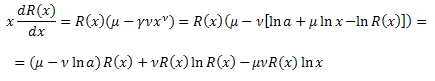
Having differentiated R(x) with respect to x, we have:
![]()
Multiply both sides by x:
![]()
Transform ![]() :
:
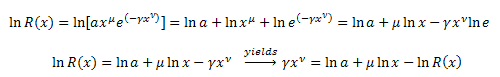
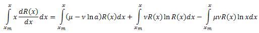
Substitute in the equation:
We obtain the differential equation for the function R(x):
![]()
Integrate both sides with respect to x over the interval [xm,x]:
Integrate the left side of the equation by parts:
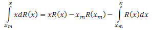
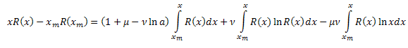
As a result, we have:
![]()
where:
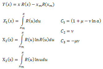
By calculating the coefficients ![]() , we can determine the function parameters
, we can determine the function parameters ![]() . The fourth parameter
. The fourth parameter ![]() can be derived from the formula for R(x).
can be derived from the formula for R(x).
2.4. Implementation
The calculation of the expansion coefficients requires to solve the system of linear equations. For convenience of working with matrices, it can be arranged as a separate class CMatrix (the CMatrix.mqh file). Using methods of this class, you can set matrix parameters, matrix element values and solve the system of linear equations employing the Gaussian method.
//+------------------------------------------------------------------+
//| CMatrix class                                                    |
//+------------------------------------------------------------------+
class CMatrix
  {
   double            m_matrix[];
   int               m_rows;
   int               m_columns;
public:
   void              SetSize(int nrows,int ncolumns);
   double            Get(int i,int j);
   void              Set(int i,int j,double val);
   void              GaussSolve(double &v[]);
   void              Test();
  };
Let us give an example of the script (EC_Example1.mq5) which calculates the eigen-coordinates and parameters of the function R(x).
//+------------------------------------------------------------------+
//|                                                  EC_Example1.mq5 |
//|                        Copyright 2012, MetaQuotes Software Corp. |
//|                                              https://www.mql5.com |
//+------------------------------------------------------------------+
#property copyright "Copyright 2012, MetaQuotes Software Corp."
#property link      "https://www.mql5.com"
#property version   "1.00"
#include <CMatrix.mqh>
//+------------------------------------------------------------------+
//| CECCalculator                                                    |
//+------------------------------------------------------------------+
class CECCalculator
  {
protected:
   int               m_size;
   //--- x[i]
   double            m_x[];
   //--- y[i]
   double            m_y[];
   //--- matrix
   CMatrix           m_matrix;
   //--- Y[i]
   double            m_ec_y[];
   //--- eigen-coordinates X1[i],X2[i],X3[i]
   double            m_ec_x1[];
   double            m_ec_x2[];
   double            m_ec_x3[];
   //--- coefficients C1,C2,C3
   double            m_ec_coefs[];
   //--- function f1=Y-C2*X2-C3*X3
   double            m_f1[];
   //--- function f2=Y-C1*X1-C3*X3
   double            m_f2[];
   //--- function f3=Y-C1*X1-C2*X2
   double            m_f3[];
private:
   //--- function for data generation
   double            R(double x,double a,double mu,double gamma,double nu);
   //--- calculation of the integral
   double            Integrate(double &x[],double &y[],int ind);
   //--- calculation of the function Y(x)
   void              CalcY(double &y[]);
   //--- calculation of the function X1(x)
   void              CalcX1(double &x1[]);
   //--- calculation of the function X2(x)
   void              CalcX2(double &x2[]);
   //--- calculation of the function X3(x)
   void              CalcX3(double &x3[]);
   //--- calculation of the correlator
   double            Correlator(int ind1,int ind2);
public:
   //--- method for generating the test function data set x[i],y[i]
   void              GenerateData(int size,double x1,double x2,double a,double mu,double gamma,double nu);
   //--- loading data from the file
   bool              LoadData(string filename);
   //--- saving data into the file
   bool              SaveData(string filename);
   //--- saving the calculation results
   void              SaveResults(string filename);
   //--- calculation of the eigen-coordinates
   void              CalcEigenCoordinates();
   //--- calculation of the linear expansion coefficients
   void              CalcEigenCoefficients();
   //--- calculation of the function parameters
   void              CalculateParameters();
   //--- calculation of the functions f1,f2,f3
   void              CalculatePlotFunctions();
  };
//+------------------------------------------------------------------+
//| Function R(x)                                                    |
//+------------------------------------------------------------------+
double CECCalculator::R(double x,double a,double mu,double gamma,double nu)
  {
   return(a*MathExp(mu*MathLog(MathAbs(x)))*MathExp(-gamma*MathExp(nu*MathLog(MathAbs(x)))));
  }
//+-----------------------------------------------------------------------+
//| Method for generating the data set x[i],y[i] of the test function R(x)|
//+-----------------------------------------------------------------------+
void CECCalculator::GenerateData(int size,double x1,double x2,double a,double mu,double gamma,double nu)
  {
   if(size<=0) return;
   if(x1>=x2) return;
   m_size=size;
   ArrayResize(m_x,m_size);
   ArrayResize(m_y,m_size);
   double delta=(x2-x1)/(m_size-1);
//---
   for(int i=0; i<m_size; i++)
     {
      m_x[i]=x1+i*delta;
      m_y[i]=R(m_x[i],a,mu,gamma,nu);
     }
  };
//+------------------------------------------------------------------+
//| Method for loading data from the .CSV file                       |
//+------------------------------------------------------------------+
bool CECCalculator::LoadData(string filename)
  {
   int filehandle=FileOpen(filename,FILE_CSV|FILE_READ|FILE_ANSI,'\r');
   if(filehandle==INVALID_HANDLE)
     {
      Alert("Error in open of file ",filename,", error",GetLastError());
      return(false);
     }
   m_size=0;
   while(!FileIsEnding(filehandle))
     {
      string str=FileReadString(filehandle);
      if(str!="")
        {
         string astr[];
         StringSplit(str,';',astr);
         if(ArraySize(astr)==2)
           {
            ArrayResize(m_x,m_size+1);
            ArrayResize(m_y,m_size+1);
            m_x[m_size]=StringToDouble(astr[0]);
            m_y[m_size]=StringToDouble(astr[1]);
            m_size++;
           }
         else
           {
            m_size=0;
            return(false);
           }
        }
     }
   FileClose(filehandle);
   return(true);
  }
//+------------------------------------------------------------------+
//| Method for saving data into the .CSV file                        |
//+------------------------------------------------------------------+
bool CECCalculator::SaveData(string filename)
  {
   if(m_size==0) return(false);
   if(ArraySize(m_x)!=ArraySize(m_y)) return(false);
   if(ArraySize(m_x)==0) return(false);
   int filehandle=FileOpen(filename,FILE_WRITE|FILE_CSV|FILE_ANSI,'\r');
   if(filehandle==INVALID_HANDLE)
     {
      Alert("Error in open of file ",filename,", error",GetLastError());
      return(false);
     }
   for(int i=0; i<ArraySize(m_x); i++)
     {
      string s=DoubleToString(m_x[i],8)+";";
      s+=DoubleToString(m_y[i],8)+";";
      s+="\r";
      FileWriteString(filehandle,s);
     }
   FileClose(filehandle);
   return(true);
  }
//+------------------------------------------------------------------+
//| Method for the calculation of the integral                       |
//+------------------------------------------------------------------+
double CECCalculator::Integrate(double &x[],double &y[],int ind)
  {
   double sum=0;
   for(int i=0; i<ind-1; i++) sum+=(x[i+1]-x[i])*(y[i+1]+y[i])*0.5;
   return(sum);
  }
//+------------------------------------------------------------------+
//| Method for the calculation of the function Y(x)                  |
//+------------------------------------------------------------------+
void CECCalculator::CalcY(double &y[])
  {
   if(m_size==0) return;
   ArrayResize(y,m_size);
   for(int i=0; i<m_size; i++) y[i]=m_x[i]*m_y[i]-m_x[0]*m_y[0];
  };
//+------------------------------------------------------------------+
//| Method for the calculation of the function X1(x)                 |
//+------------------------------------------------------------------+
void CECCalculator::CalcX1(double &x1[])
  {
   if(m_size==0) return;
   ArrayResize(x1,m_size);
   for(int i=0; i<m_size; i++) x1[i]=Integrate(m_x,m_y,i);
  }
//+------------------------------------------------------------------+
//| Method for the calculation of the function X2(x)                 |
//+------------------------------------------------------------------+
void CECCalculator::CalcX2(double &x2[])
  {
   if(m_size==0) return;
   double tmp[];
   ArrayResize(tmp,m_size);
   for(int i=0; i<m_size; i++) tmp[i]=m_y[i]*MathLog(MathAbs(m_y[i]));
   ArrayResize(x2,m_size);
   for(int i=0; i<m_size; i++) x2[i]=Integrate(m_x,tmp,i);
  }
//+------------------------------------------------------------------+
//| Method for the calculation of the function X3(x)                 |
//+------------------------------------------------------------------+
void CECCalculator::CalcX3(double &x3[])
  {
   if(m_size==0) return;
   double tmp[];
   ArrayResize(tmp,m_size);
   for(int i=0; i<m_size; i++) tmp[i]=m_y[i]*MathLog(MathAbs(m_x[i]));
   ArrayResize(x3,m_size);
   for(int i=0; i<m_size; i++) x3[i]=Integrate(m_x,tmp,i);
  }
//+------------------------------------------------------------------+
//| Method for the calculation of the eigen-coordinates              |
//+------------------------------------------------------------------+
void CECCalculator::CalcEigenCoordinates()
  {
   CalcY(m_ec_y);
   CalcX1(m_ec_x1);
   CalcX2(m_ec_x2);
   CalcX3(m_ec_x3);
  }
//+------------------------------------------------------------------+
//| Method for the calculation of the correlator                     |
//+------------------------------------------------------------------+
double CECCalculator::Correlator(int ind1,int ind2)
  {
   if(m_size==0) return(0);
   if(ind1<=0 || ind1>4) return(0);
   if(ind2<=0 || ind2>4) return(0);
//---
   double arr1[];
   double arr2[];
   ArrayResize(arr1,m_size);
   ArrayResize(arr2,m_size);
//---
   switch(ind1)
     {
      case 1: ArrayCopy(arr1,m_ec_x1,0,0,WHOLE_ARRAY); break;
      case 2: ArrayCopy(arr1,m_ec_x2,0,0,WHOLE_ARRAY); break;
      case 3: ArrayCopy(arr1,m_ec_x3,0,0,WHOLE_ARRAY); break;
      case 4: ArrayCopy(arr1,m_ec_y,0,0,WHOLE_ARRAY); break;
     }
   switch(ind2)
     {
      case 1: ArrayCopy(arr2,m_ec_x1,0,0,WHOLE_ARRAY); break;
      case 2: ArrayCopy(arr2,m_ec_x2,0,0,WHOLE_ARRAY); break;
      case 3: ArrayCopy(arr2,m_ec_x3,0,0,WHOLE_ARRAY); break;
      case 4: ArrayCopy(arr2,m_ec_y,0,0,WHOLE_ARRAY); break;
     }
//---
   double sum=0;
   for(int i=0; i<m_size; i++) { sum+=arr1[i]*arr2[i];  }
   sum=sum/m_size;
   return(sum);
  };
//+------------------------------------------------------------------+
//| Method for the calculation of the linear expansion coefficients  |
//+------------------------------------------------------------------+
void CECCalculator::CalcEigenCoefficients()
  {
//--- setting the matrix size 3x4
   m_matrix.SetSize(3,4);
//--- calculation of the correlation matrix
   for(int i=3; i>=1; i--)
     {
      string s="";
      for(int j=1; j<=4; j++)
        {
         double corr=Correlator(i,j);
         m_matrix.Set(i,j,corr);
         s=s+" "+DoubleToString(m_matrix.Get(i,j));
        }
      Print(i," ",s);
     }
//--- solving the system of the linear equations
   m_matrix.GaussSolve(m_ec_coefs);
//--- displaying the solution - the obtained coefficients C1,..CN
   for(int i=ArraySize(m_ec_coefs)-1; i>=0; i--) Print("C",i+1,"=",m_ec_coefs[i]);
  };
//+--------------------------------------------------------------------+
//| Method for the calculation of the function parameters a,mu,nu,gamma|
//+--------------------------------------------------------------------+
void CECCalculator::CalculateParameters()
  {
   if(ArraySize(m_ec_coefs)==0) {Print("Coefficients are not calculated!"); return;}
//--- calculate a
   double a=MathExp((1-m_ec_coefs[0])/m_ec_coefs[1]-m_ec_coefs[2]/(m_ec_coefs[1]*m_ec_coefs[1]));
//--- calculate mu
   double mu=-m_ec_coefs[2]/m_ec_coefs[1];
//--- calculate nu
   double nu=m_ec_coefs[1];
//--- calculate gamma
   double arr1[],arr2[];
   ArrayResize(arr1,m_size);
   ArrayResize(arr2,m_size);
   double corr1=0;
   double corr2=0;
   for(int i=0; i<m_size; i++)
     {
      arr1[i]=MathPow(m_x[i],nu);
      arr2[i]=MathLog(MathAbs(m_y[i]))-MathLog(a)-mu*MathLog(m_x[i]);
      corr1+=arr1[i]*arr2[i];
      corr2+=arr1[i]*arr1[i];
     }
   double gamma=-corr1/corr2;
//---
   Print("a=",a);
   Print("mu=",mu);
   Print("nu=",nu);
   Print("gamma=",gamma);
  };
//+------------------------------------------------------------------+
//| Method for the calculation of the functions                      |
//| f1=Y-C2*X2-C3*X3                                                 |
//| f2=Y-C1*X1-C3*X3                                                 |
//| f3=Y-C1*X1-C2*X2                                                 |
//+------------------------------------------------------------------+
void CECCalculator::CalculatePlotFunctions()
  {
   if(ArraySize(m_ec_coefs)==0) {Print("Coefficients are not calculated!"); return;}
//---
   ArrayResize(m_f1,m_size);
   ArrayResize(m_f2,m_size);
   ArrayResize(m_f3,m_size);
//---
   for(int i=0; i<m_size; i++)
     {
      //--- plot function f1=Y-C2*X2-C3*X3
      m_f1[i]=m_ec_y[i]-m_ec_coefs[1]*m_ec_x2[i]-m_ec_coefs[2]*m_ec_x3[i];
      //--- plot function f2=Y-C1*X1-C3*X3
      m_f2[i]=m_ec_y[i]-m_ec_coefs[0]*m_ec_x1[i]-m_ec_coefs[2]*m_ec_x3[i];
      //--- plot function f3=Y-C1*X1-C2*X2
      m_f3[i]=m_ec_y[i]-m_ec_coefs[0]*m_ec_x1[i]-m_ec_coefs[1]*m_ec_x2[i];
     }
  }
//+------------------------------------------------------------------+
//| Method for saving the calculation results                        |
//+------------------------------------------------------------------+
void CECCalculator::SaveResults(string filename)
  {
   if(m_size==0) return;
   int filehandle=FileOpen(filename,FILE_WRITE|FILE_CSV|FILE_ANSI);
   if(filehandle==INVALID_HANDLE)
     {
      Alert("Error in open of file ",filename," for writing, error",GetLastError());
      return;
     }
   for(int i=0; i<m_size; i++)
     {
      string s=DoubleToString(m_x[i],8)+";";
      s+=DoubleToString(m_y[i],8)+";";
      s+=DoubleToString(m_ec_y[i],8)+";";
      s+=DoubleToString(m_ec_x1[i],8)+";";
      s+=DoubleToString(m_f1[i],8)+";";
      s+=DoubleToString(m_ec_x2[i],8)+";";
      s+=DoubleToString(m_f2[i],8)+";";
      s+=DoubleToString(m_ec_x3[i],8)+";";
      s+=DoubleToString(m_f3[i],8)+";";
      s+="\r";
      FileWriteString(filehandle,s);
     }
   FileClose(filehandle);
  }
//+------------------------------------------------------------------+
//| Script program start function                                    |
//+------------------------------------------------------------------+
void OnStart()
  {
   CECCalculator ec;
//--- model function data preparation
   ec.GenerateData(100,0.25,15.25,1.55,1.05,0.15,1.3);
//--- saving into the file
   ec.SaveData("ex1.csv");
//--- calculation of the eigen-coordinates
   ec.CalcEigenCoordinates();
//--- calculation of the coefficients
   ec.CalcEigenCoefficients();
//--- calculation of the parameters
   ec.CalculateParameters();
//--- calculation of the functions f1,f2,f3
   ec.CalculatePlotFunctions();
//--- saving the results into the file
   ec.SaveResults("ex1-results.csv");
  }
2.5. The R(x) Model Function Calculation Results
We will generate 100 values of the R(x) function over the interval [0.25,15.25] as the model data

Fig. 7. Model function used for calculations
These data provide the basis for plotting the function Y(x) and its expansion in the functions X1(x), X2(x) and X3(x).
Fig. 8 shows the function Y(x) and its "eigen-coordinates" X1(x), X2(x) and X3(x).
 and the eigen-coordinates X1(x), X2(x) and X3(x)")
Fig. 8. General form of the function Y(x) and the eigen-coordinates X1(x), X2(x) and X3(x)
Note the smoothness of these functions resulting from integral nature of the operators X1(x), X2(x) and X3(x).
Following the calculation of the functions Y(x), X1(x), X2(x) and X3(x), the correlation matrix is constructed, then the equations for the coefficients C1, C2 and C3 are solved and the R(x) function parameters are calculated based on the values obtained:
2012.06.21 14:20:28 ec_example1 (EURUSD,H1) gamma=0.2769402213886906
2012.06.21 14:20:28 ec_example1 (EURUSD,H1) nu=1.126643424450548
2012.06.21 14:20:28 ec_example1 (EURUSD,H1) mu=1.328595266178149
2012.06.21 14:20:28 ec_example1 (EURUSD,H1) a=1.637687667818532
2012.06.21 14:20:28 ec_example1 (EURUSD,H1) C1=1.772838639779728
2012.06.21 14:20:28 ec_example1 (EURUSD,H1) C2=1.126643424450548
2012.06.21 14:20:28 ec_example1 (EURUSD,H1) C3=-1.496853120395737
2012.06.21 14:20:28 ec_example1 (EURUSD,H1) 1  221.03637620 148.53278281 305.48547011 101.93843241
2012.06.21 14:20:28 ec_example1 (EURUSD,H1) 2  148.53278281 101.63995012 202.85142688 74.19784681
2012.06.21 14:20:28 ec_example1 (EURUSD,H1) 3  305.48547011 202.85142688 429.09345292 127.82779760
We will now check for linearity of the expansion calculated. For this purpose, we need to calculate 3 functions:
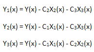
each of which is projected on its basis of the eigen-coordinates X1(x), X2(x) and X3(x):
 in the basis X1(x)")
Fig. 9. Representation of the function Y1(x) in the basis X1(x)
 in the basis X2(x)")
Fig. 10. Representation of the function Y2(x) in the basis X2(x)
 in the basis X3(x)")
Fig. 11. Representation of the function Y3(x) in the basis X3(x)
The linear dependence of the plotted functions suggests that the data series in Fig. 7 strictly corresponds to the function R(x).
Any other function (even similar in form) represented in the R(x) eigen-coordinates will no longer have a linear form. This fact enables us to identify functions.
The accuracy of the calculation of numerical values of the model function parameters can be improved, if the number of points is increased to 10000 (while keeping the same interval):
2012.06.21 14:22:18 ec_example1 (EURUSD,H1) gamma=0.1508739336762316
2012.06.21 14:22:18 ec_example1 (EURUSD,H1) nu=1.298316173744703
2012.06.21 14:22:18 ec_example1 (EURUSD,H1) mu=1.052364487161627
2012.06.21 14:22:18 ec_example1 (EURUSD,H1) a=1.550281229466634
2012.06.21 14:22:18 ec_example1 (EURUSD,H1) C1=1.483135479113404
2012.06.21 14:22:18 ec_example1 (EURUSD,H1) C2=1.298316173744703
2012.06.21 14:22:18 ec_example1 (EURUSD,H1) C3=-1.36630183435649
2012.06.21 14:22:18 ec_example1 (EURUSD,H1) 1  225.47846911 151.22066473 311.86134419 104.65062550
2012.06.21 14:22:18 ec_example1 (EURUSD,H1) 2  151.22066473 103.30005101 206.66297964 76.03285182
2012.06.21 14:22:18 ec_example1 (EURUSD,H1) 3  311.86134419 206.66297964 438.35625824 131.91955339
In this case, the function parameters have been calculated more accurately.
2.6. Noise Effect
Real experimental data always contain noise.
In the GenerateData() method of the ECCCalculator class, we replace:
m_y[i]=R(m_x[i],a,mu,gamma,nu);
with
m_y[i]=R(m_x[i],a,mu,gamma,nu)+0.25*MathRand()/32767.0;
adding a random noise, being approximately 10% of the maximum function value.
The EC_Example1-noise.mq5 script result is as follows:
2012.06.21 14:24:30 EC_Example1-noise (EURUSD,H1) gamma=0.4013079343855266
2012.06.21 14:24:30 EC_Example1-noise (EURUSD,H1) nu=0.9915044018913447
2012.06.21 14:24:30 EC_Example1-noise (EURUSD,H1) mu=1.403541951457922
2012.06.21 14:24:30 EC_Example1-noise (EURUSD,H1) a=2.017238416806171
2012.06.21 14:24:30 EC_Example1-noise (EURUSD,H1) C1=1.707774107235756
2012.06.21 14:24:30 EC_Example1-noise (EURUSD,H1) C2=0.9915044018913447
2012.06.21 14:24:30 EC_Example1-noise (EURUSD,H1) C3=-1.391618023109698
2012.06.21 14:24:30 EC_Example1-noise (EURUSD,H1) 1  254.45082565 185.19087989 354.25574000 125.17343164
2012.06.21 14:24:30 EC_Example1-noise (EURUSD,H1) 2  185.19087989 136.81028987 254.92996885 97.14705491
2012.06.21 14:24:30 EC_Example1-noise (EURUSD,H1) 3  354.25574000 254.92996885 501.76021715 159.49440494
The chart of the model function with a random noise is demonstrated in Fig. 12.

Fig. 12. Model function with noise used for calculations
 and the eigen-coordinates X1(x), X2(x) and X3(x)")
Fig. 13. General form of the function Y(x) and the eigen-coordinates X1(x), X2(x) and X3(x)
The functions X1(x), X2(x) and X3(x) serving as the "eigen-coordinates" still look smooth, however the Y(x) plotted as their linear combination appears to be different (Fig. 13).
 in the basis X1(x)")
Fig. 14. Representation of the function Y1(x) in the basis X1(x)
 in the basis X2(x)")
Fig. 15. Representation of the function Y2(x) in the basis X2(x)
 in the basis X3(x)")
Fig. 16. Representation of the function Y3(x) in the basis X3(x)
The representation of the functions Y1(x),Y2(x) and Y3(x) in the basis of the eigen-coordinates (Figures 8-10) still has a linear form yet one can notice fluctuations around the straight line due to the presence of noise. It is most pronounced with respect to greater X's where the signal/noise becomes minimal.
Here, the noise components are lying on both sides of the straight line and in this case it is therefore convenient to use the integral eigen-coordinates expansion (Section 2.2).
3. Nonextensive Probability Distributions
The generalization of statistical mechanics results in the distributions [2, 22]:
![]()
![]()
where ![]() ,
, ![]() .
.
The q-Gaussian distribution is a special case of the function P2(x).
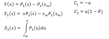
3.1. The P1(x) Function Eigen-Coordinates Expansion
We differentiate P1(x):
![]()
The resulting differential equation is as follows:
![]()
![]()
Integrate over the interval [xm,x]:
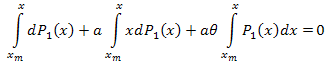
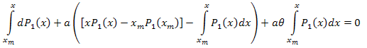
Thus:
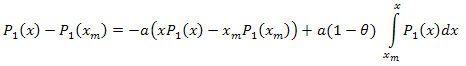
The eigen-coordinates expansion is as follows:
![]()
where:
The functions for calculations are as set forth below (EC_Example2.mq5):
//+------------------------------------------------------------------+
//| CalcY                                                            |
//+------------------------------------------------------------------+
void CECCalculator::CalcY(double &y[])
  {
   if(m_size==0) return;
   ArrayResize(y,m_size);
//--- Y=P(x)-P(xm)
   for(int i=0; i<m_size; i++) y[i]=m_y[i]-m_y[0];
  };
//+------------------------------------------------------------------+
//| CalcX1                                                           |
//+------------------------------------------------------------------+
void CECCalculator::CalcX1(double &x1[])
  {
   if(m_size==0) return;
   ArrayResize(x1,m_size);
//--- X1=x*P(x)-xm*P(xm)
   for(int i=0; i<m_size; i++) x1[i]=m_x[i]*m_y[i]-m_x[0]*m_y[0];
  }
//+------------------------------------------------------------------+
//| CalcX2                                                           |
//+------------------------------------------------------------------+
void CECCalculator::CalcX2(double &x2[])
  {
   if(m_size==0) return;
   ArrayResize(x2,m_size);
//--- X2=Integrate(P1(x))
   for(int i=0; i<m_size; i++) x2[i]=Integrate(m_x,m_y,i);
  }
This time the correlation matrix size is 2x3; the values of the parameters a and theta of the P1(x) function are determined based on the coefficients С1 and C2. The numerical value of the parameter B can be obtained from the normalization requirement.
Below is the P1(x,1,0.5,2) model function calculation result over the interval x [0,10]; the number of points used is 1000:
2012.06.21 14:26:02 EC_Example2 (EURUSD,H1) theta=1.986651299600245
2012.06.21 14:26:02 EC_Example2 (EURUSD,H1) a=0.5056083906174813
2012.06.21 14:26:02 EC_Example2 (EURUSD,H1) C1=-0.5056083906174813
2012.06.21 14:26:02 EC_Example2 (EURUSD,H1) C2=-0.4988591756915261
2012.06.21 14:26:02 EC_Example2 (EURUSD,H1) 1  0.15420524 0.48808959 -0.32145543
2012.06.21 14:26:02 EC_Example2 (EURUSD,H1) 2  0.48808959 1.79668322 -1.14307410
The function P1(x) and its eigen-coordinates expansion are shown in Figures 17-20.
 used for calculations, 1000 points")
Fig. 17. Model function P1(x, 1, 0.5, 2) used for calculations, 1000 points
 and the eigen-coordinates X1(x) and X2(x)")
Fig. 18. General form of the function Y(x) and the eigen-coordinates X1(x) and X2(x)
 in the basis X1(x)")
Fig. 19. Representation of the function Y1(x) in the basis X1(x)
 in the basis X2(x)")
Fig. 20. Representation of the function Y2(x) in the basis X2(x)
Take a close look at the Fig. 19. There is a slight distortion of the linear dependence at the very beginning and in the second third of the chart.
This is associated with the peculiarities of the expansion calculated - X1(x) is not of integral nature.
3.2. The P2(x) Function Eigen-Coordinates Expansion
![]()

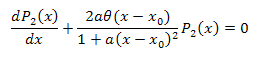
The differential equation:
![]()

We integrate with respect to x over the interval [xm,x]:
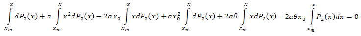

Integrating by parts, we have:

Simplify:
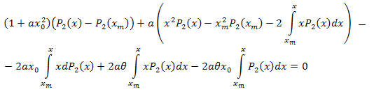
Following the algebraic manipulations, we get:
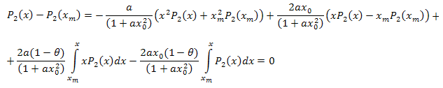
Thus, the resulting expansion is as follows:
![]()
where:
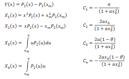
The function parameters can be calculated using the formulas below:
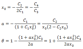
It should be noted that there is an additional relationship between the parameters in the resulting expansion. This fact can be used to verify the correctness of the function selected for the analysis. These relationships are always true for the data strictly corresponding to the function P2(x).
The numerical value of the parameter B can be obtained from the normalization requirement.
The functions for the calculation of the eigen-coordinates are as follows (EC_Example3.mq5):
//+------------------------------------------------------------------+
//| CalcY                                                            |
//+------------------------------------------------------------------+
void CECCalculator::CalcY(double &y[])
  {
   if(m_size==0) return;
   ArrayResize(y,m_size);
   for(int i=0; i<m_size; i++) y[i]=m_y[i]-m_y[0];
  };
//+------------------------------------------------------------------+
//| CalcX1                                                           |
//+------------------------------------------------------------------+
void CECCalculator::CalcX1(double &x1[])
  {
   if(m_size==0) return;
   ArrayResize(x1,m_size);
   //--- X1=(x^2)*P2(x)+(xm)^2*P2(xm)
   for(int i=0; i<m_size; i++) x1[i]=(m_x[i]*m_x[i])*m_y[i]+(m_x[0]*m_x[0])*m_y[0];
  }
//+------------------------------------------------------------------+
//| CalcX2                                                           |
//+------------------------------------------------------------------+
void CECCalculator::CalcX2(double &x2[])
  {
   if(m_size==0) return;
   ArrayResize(x2,m_size);
   //--- X2=(x)*P2(x)-(xm)*P2(xm)
   for(int i=0; i<m_size; i++) x2[i]=m_x[i]*m_y[i]-m_x[0]*m_y[0];
  }
//+------------------------------------------------------------------+
//| CalcX3                                                           |
//+------------------------------------------------------------------+
void CECCalculator::CalcX3(double &x3[])
  {
   if(m_size==0) return;
   double tmp[];
   ArrayResize(tmp,m_size);
   for(int i=0; i<m_size; i++) tmp[i]=m_x[i]*m_y[i];
   //--- X3=Integrate(X*P2(x))
   ArrayResize(x3,m_size);
   for(int i=0; i<m_size; i++) x3[i]=Integrate(m_x,tmp,i);
  }
//+------------------------------------------------------------------+
//| CalcX4                                                           |
//+------------------------------------------------------------------+
void CECCalculator::CalcX4(double &x4[])
  {
   if(m_size==0) return;
   //--- X4=Integrate(P2(x))
   ArrayResize(x4,m_size);
   for(int i=0; i<m_size; i++) x4[i]=Integrate(m_x,m_y,i);
  }
Below is the P2(x) model function calculation result (B=1, a=0.5, theta=2, x0=1); the number of point used is 1000:
2012.06.21 14:27:47 EC_Example3 (EURUSD,H1) 2: theta=2.260782711057654
2012.06.21 14:27:47 EC_Example3 (EURUSD,H1) 1: theta=2.076195813531546
2012.06.21 14:27:47 EC_Example3 (EURUSD,H1) 2: a=0.4557937139014854
2012.06.21 14:27:47 EC_Example3 (EURUSD,H1) 1: a=0.4977821155774935
2012.06.21 14:27:47 EC_Example3 (EURUSD,H1) 2: x0=1.043759816231049
2012.06.21 14:27:47 EC_Example3 (EURUSD,H1) 1: x0=0.8909465007003451
2012.06.21 14:27:47 EC_Example3 (EURUSD,H1) C1=-0.3567992171618368
2012.06.21 14:27:47 EC_Example3 (EURUSD,H1) C2=0.6357780279659221
2012.06.21 14:27:47 EC_Example3 (EURUSD,H1) C3=-0.7679716475618039
2012.06.21 14:27:47 EC_Example3 (EURUSD,H1) C4=0.8015779457297644
2012.06.21 14:27:47 EC_Example3 (EURUSD,H1) 1  1.11765877 0.60684314 1.34789126 1.28971267 -0.01429928
2012.06.21 14:27:47 EC_Example3 (EURUSD,H1) 2  0.60684314 0.37995888 0.55974145 0.58899739 0.06731011
2012.06.21 14:27:47 EC_Example3 (EURUSD,H1) 3  1.34789126 0.55974145 3.00225771 2.54531927 -0.39043224
2012.06.21 14:27:47 EC_Example3 (EURUSD,H1) 4  1.28971267 0.58899739 2.54531927 2.20595917 -0.27218168
The function P2(x) and its eigen-coordinates expansion are shown in Figures 21-26.
 used for calculations, 100 points")
Fig. 21. Model function P2(x,1,0.5,2,1) used for calculations, 100 points
 and the eigen-coordinates X1(x), X2(x), X3(x) and X4(x)")
Fig. 22. General form of the function Y(x) and the eigen-coordinates X1(x), X2(x), X3(x) and X4(x)
 in the basis X1(x)")
Fig. 23. Representation of the function Y1(x) in the basis X1(x)
 in the basis X2(x)")
Fig. 24. Representation of the function Y2(x) in the basis X2(x)
 in the basis X3(x)")
Fig. 25. Representation of the function Y3(x) in the basis X3(x)
 in the basis X4(x)")
Fig. 26. Representation of the function Y4(x) in the basis X4(x)
4. If It Looks Like a Cat... It Might Not Be a Cat
The family of the q-Gaussian distributions lies at the very heart of nonextensive statistical mechanics and it was therefore natural to expect that it would appear in the generalized central limit theorem. Entropic considerations served as the main argument in its favor [26].
However, the article [18, presentation] showed that distributions, such as the q-Gaussian, are not universal, thus casting doubt on their special role as limit distributions.
For example, the function (analytical solution to one of the problems):
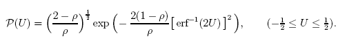
can be very accurately described using the q-Gaussian distribution.

Fig. 27. An example from the article "A Note on q-Gaussians and Non-Gaussians in Statistical Mechanics"
In this case, analytically different functions have similar numerical values and the differences are therefore barely visible to the eye. An accurate function identification method is required. This problem can be nicely solved using the eigen-coordinates method.
Let us review an example of the P(U) function eigen-coordinates expansion and show what exactly makes it different from the q-Gaussian. The functions appear very similar to the eye (Fig. 27).
We generate a signal (100 values of the P(U) function) and "project" it on the system of the eigen-coordinates of the P2(x) function plotted in Section 3.2.
The Hilhorst-Schehr-problem.mq5 script calculates the P(U) function and constructs data series which is saved in the MQL5\Files\test-data.csv file. These data are analyzed by EC_Example3_Test.mq5.
, 100 points")
Fig. 28. Model function P(U), 100 points
 and the eigen-coordinates X1(x), X2(x), X3(x) and X4(x)")
Fig. 29. General form of the function Y(x) and the eigen-coordinates X1(x), X2(x), X3(x) and X4(x)
 in the basis X1(x)")
Fig. 30. Representation of the function Y1(x) in the basis X1(x)
 in the basis X2(x)")
Fig. 31. Representation of the function Y2(x) in the basis X2(x)
 in the basis X3(x)")
Fig. 32. Representation of the function Y3(x) in the basis X3(x)
 in the basis X4(x)")
Fig. 33. Representation of the function Y4(x) in the basis X4(x)
As Fig. 30-33 suggest, the functions P2(x) and P(U) are very similar in terms of the coordinates X1(x), X2(x) and X3(x) - one can observe a good linear dependence between Xi(x) and Yi(x). A significant difference can be seen in the X4(x) component (Fig. 33).
The absence of the linear dependence for the X4(x) component proves the fact that the data set generated by P(U), in spite of appearing similar to the q-Gaussian distribution, is in fact not the q-Gaussian.
We can take a different look at the functions (Figures 34-37) by plotting Xi(x) and Yi(x) together.
 and Y1(x)")
Fig. 34. General form of the functions X1(x) and Y1(x)
 and Y2(x)")
Fig. 35. General form of the functions X2(x) and Y2(x)
 and Y3(x)")
Fig. 36. General form of the functions X3(x) and Y3(x)
 and Y4(x)")
Fig. 37. General form of the functions X4(x) and Y4(x)
As Fig. 37 suggests, the structural difference in the X4(x) component has become apparent when projecting data generated by the P(U) function on the eigen-coordinates of the P2(x) function. Thus, we can say for certain that the experimental data do not correspond to the P2(x) function.
The calculation set forth below (EC_Example3_test) speaks in favor of this fact:
2012.06.21 14:29:35 EC_Example3_test (EURUSD,H1) 2: theta=1.034054797050629
2012.06.21 14:29:35 EC_Example3_test (EURUSD,H1) 1: theta=-0.6736146397139184
2012.06.21 14:29:35 EC_Example3_test (EURUSD,H1) 2: a=199.3574440289263
2012.06.21 14:29:35 EC_Example3_test (EURUSD,H1) 1: a=-4.052181367572913
2012.06.21 14:29:35 EC_Example3_test (EURUSD,H1) 2: x0=-0.0003278538628371299
2012.06.21 14:29:35 EC_Example3_test (EURUSD,H1) 1: x0=0.0161122975924721
2012.06.21 14:29:35 EC_Example3_test (EURUSD,H1) C1=4.056448634458822
2012.06.21 14:29:35 EC_Example3_test (EURUSD,H1) C2=-0.1307174151339552
2012.06.21 14:29:35 EC_Example3_test (EURUSD,H1) C3=-13.57786363975563
2012.06.21 14:29:35 EC_Example3_test (EURUSD,H1) C4=-0.004451555043369697
2012.06.21 14:29:35 EC_Example3_test (EURUSD,H1) 1  0.00465975 0.00000000 -0.00218260 0.02762761 0.04841405
2012.06.21 14:29:35 EC_Example3_test (EURUSD,H1) 2  0.00000000 0.04841405 -0.00048835 0.06788438 0.00000001
2012.06.21 14:29:35 EC_Example3_test (EURUSD,H1) 3  -0.00218260 -0.00048835 0.00436149 -0.02811625 -0.06788437
2012.06.21 14:29:35 EC_Example3_test (EURUSD,H1) 4  0.02762761 0.06788438 -0.02811625 0.35379820 0.48337994
It has also impaired the relationships between the parameters.
Conclusion
The eigen-coordinates method is a unique tool for the analysis of structural properties of functional relationships allowing to substantially simplify the analysis and interpretation of data.
The concept behind this method is to use experimental data sets {xi,yi} to build new functions corresponding to the proposed model. The form of operator expansions is determined by the structure of the differential equation which is satisfied by the function serving as a "candidate" for the description of data. If the function is native, the function expansions calculated using the data {xi,yi}, will in the basis of the eigen-coordinates take a linear form. Deviations from linearity in the basis of the eigen-coordinates of the "candidate function" suggest that the data {xi,yi} could not be generated by the given function and the model built is not appropriate.
In some complicated cases the candidate function and the native function may appear similar insomuch that a bigger part of the calculated expansions turns out to be linear. Nevertheless, the eigen-coordinates method enables us to identify the difference between these functions which makes its presence known by impaired linearity of the expansion - the example by Hilhorst and Schehr has served as an illustration of the difference becoming apparent in the last expansion member when projecting on X4(x).
This information can also be useful when dealing with a differential equation (Section 3.2) which is satisfied by the function P2(x) - the member in question corresponds to the linear part with respect to P2(x). It may not be so interesting in case of phenomenological description of experimental data ("we are looking for a solution in the form of the q-Gaussian"). However if the model is based on differential equations (Fig. 3), the role of each of the mechanisms taken into consideration in models of physical processes can be better understood.
References
- C. Tsallis, "Possible Generalization of Boltzmann-Gibbs Statistics", Journal of Statistical Physics, Vol. 52, Nos. 1/2, 1988.
- C. Tsallis, "Nonextensive Statistics: Theoretical, Experimental and Computational Evidences and Connections". Brazilian Journal of Physics, (1999) vol. 29. p.1.
- C. Tsallis, "Some Comments on Boltzmann-Gibbs Statistical Mechanics", Chaos, Solitons & Fractals Volume 6, 1995, pp. 539–559.
- Europhysics News "Special Issue: Nonextensive Statistical Mechanics: New Trends, New Perspectives", Vol. 36 No. 6 (November-December 2005).
- M. Gell-Mann, C. Tsallis, "Nonextensive Entropy: Interdisciplinary Applications", Oxford University Press, 15.04.2004, 422 p.
- Constantino Tsallis, the Official Website Nonextensive Statistical Mechanics and Thermodynamics.
- Chumak, O.V. "Entropy and Fractals in Data Analysis", М.-Izhevsk: RDC "Regular and Chaotic Dynamics", Institute for Computer Research, 2011. - 164 p.
- Qiuping A. Wang, "Incomplete Statistics and Nonextensive Generalizations of Statistical Mechanics", Chaos, Solitons and Fractals, 12(2001)1431-1437.
- Qiuping A. Wang, "Extensive Generalization of Statistical Mechanics Based on Incomplete Information Theory", Entropy, 5(2003).
- Lisa Borland, "Long-Range Memory and Nonextensivity in Financial Markets", Europhysics News 36, 228-231 (2005)
- T. S. Biró, R. Rosenfeld, "Microscopic Origin of Non-Gaussian Distributions of Financial Returns", Physica A: Statistical Mechanics and its Applications, Vol. 387, Nr. 7 (Mar 1, 2008) , p. 1603-1612 (preprint).
- S. M. D. Queiros, C. Anteneodo, C. Tsallis, "Power-Law Distributions in Economics: A Nonextensive Statistical Approach", Proceedings of SPIE (2005) Volume: 5848, Publisher: SPIE, Pages: 151-164, (preprint)
- R Hanel, S Thurner, "Derivation of Power-Law Distributions within Standard Statistical Mechanics", Physica A: Statistical Mechanics and its Applications (2005), Volume: 351, Issue: 2-4, Publisher: Elsevier, Pages: 260-268. (preprint)
- A K Rajagopal, Sumiyoshi Abe, "Statistical Mechanical Foundations of Power-Law Distributions", Physica D: Nonlinear Phenomena (2003), Volume: 193, Issue: 1-4, Pages: 19 (preprint)
- T. Kaizoji, "An Interacting-Agent Model of Financial Markets from the Viewpoint of Nonextensive Statistical Mechanics", Physica A: Statistical Mechanics and its Applications, Vol. 370, N. 1 (Oct 1, 2006) , p. 109-113. (preprint)
- V. Gontis, J. Ruseckas, A. Kononovičius, "A Long-Range Memory Stochastic Model of the Return in Financial Markets", Physica A: Statistical Mechanics and its Applications 389 (2010) 100-106. (preprint)
- H.E. Roman, M. Porto, "Self-Generated Power-Law Tails in Probability Distributions", Physical Review E - Statistical, Nonlinear and Soft Matter Physics (2001), Volume: 63, Issue: 3 Pt 2, Pages: 036-128.
- H. J. Hilhorst, G. Schehr, "A Note on q-Gaussians and Non-Gaussians in Statistical Mechanics" (2007, preprint, presentation).
- D. J. Hudson, "Lectures on Elementary Statistics and Probability", CERN-63-29, Geneva : CERN, 1963. - 101 p.
- D. J. Hudson, "Statistics Lectures II : Maximum Likelihood and Least Squares Theory", CERN-64-18. - Geneva : CERN, 1964. - 115 p.
- R. R. Nigmatullin, "Eigen-Coordinates: New Method of Analytical Functions Identification in Experimental Measurements", Applied Magnetic Resonance Volume 14, Number 4 (1998), 601-633.
- R.R. Nigmatullin, "Recognition of Nonextensive Statistical Distributions by the Eigencoordinates Method", Physica A: Statistical Mechanics and its Applications Volume 285, Issues 3–4, 1 October 2000, pp. 547–565.
- C. Antonini "q-Gaussians in Finance" (2010).
- C. Antonini, "The Use of the q-Gaussian Distribution in Finance" (2011).
- L. G. Moyano, C. Tsallis, M. Gell-Mann, "Numerical Indications of a q-Generalised Central Limit Theorem", Europhysics Letters 73, 813-819, 2006, (preprint).
- T. Dauxois, "Non-Gaussian Distributions under Scrutiny", J. Stat. Mech. (2007) N08001. (preprint)
Appendix. Analysis of SP500 daily returns with Q-Gaussian
Let us consider classical example (Fig. 4) of successful q-Gaussian approach to SP500 daily returns(P2(x) function).
We have used the daily data from: http://wikiposit.org/w?filter=Finance/Futures/Indices/S__and__P%20500/
")
Fig. 38. SP500 close prices (daily)

Fig. 39. SP500 logarithmic returns

Fig. 40. SP500 logarithmic returns distribution
 in basis X1(x)")
Fig. 41. The function Y1(x) in basis X1(x)
 in basis X2(x)")
Fig. 42. The function Y2(x) in basis X2(x)
 in basis X3(x)")
Fig. 43. The function Y3(x) in basis X3(x)
 in basis X4(x))")
Fig. 44. The function Y4(x) in basis X4(x)
To see how to perform the analysis in your terminal, the file SP500-data.csv must be placed to \Files\ folder.
After that you need to launch two scripts:
- CalcDistr_SP500.mq5 (it calculates the distribution).
- q-gaussian-SP500.mq5 (eigen-coordinates analysis)
2012.06.29 20:01:19    q-gaussian-SP500 (EURUSD,D1)    2: theta=1.770125768485269
2012.06.29 20:01:19    q-gaussian-SP500 (EURUSD,D1)    1: theta=1.864132228192338
2012.06.29 20:01:19    q-gaussian-SP500 (EURUSD,D1)    2: a=2798.166930885822
2012.06.29 20:01:19    q-gaussian-SP500 (EURUSD,D1)    1: a=8676.207867097581
2012.06.29 20:01:19    q-gaussian-SP500 (EURUSD,D1)    2: x0=0.04567518783335043
2012.06.29 20:01:19    q-gaussian-SP500 (EURUSD,D1)    1: x0=0.0512505923716428
2012.06.29 20:01:19    q-gaussian-SP500 (EURUSD,D1)    C1=-364.7131366394939
2012.06.29 20:01:19    q-gaussian-SP500 (EURUSD,D1)    C2=37.38352859698793
2012.06.29 20:01:19    q-gaussian-SP500 (EURUSD,D1)    C3=-630.3207508306047
2012.06.29 20:01:19    q-gaussian-SP500 (EURUSD,D1)    C4=28.79001868944634
2012.06.29 20:01:19    q-gaussian-SP500 (EURUSD,D1)    1  0.00177913 0.03169294 0.00089521 0.02099064 0.57597695
2012.06.29 20:01:19    q-gaussian-SP500 (EURUSD,D1)    2  0.03169294 0.59791579 0.01177430 0.28437712 11.55900584
2012.06.29 20:01:19    q-gaussian-SP500 (EURUSD,D1)    3  0.00089521 0.01177430 0.00193200 0.04269286 0.12501732
2012.06.29 20:01:19    q-gaussian-SP500 (EURUSD,D1)    4  0.02099064 0.28437712 0.04269286 0.94465120 3.26179090
2012.06.29 20:01:09    CalcDistr_SP500 (EURUSD,D1)    checking distibution cnt=2632.0 n=2632
2012.06.29 20:01:09    CalcDistr_SP500 (EURUSD,D1)    Min=-0.1229089015984444 Max=0.1690557338964631 range=0.2919646354949075 size=2632
2012.06.29 20:01:09    CalcDistr_SP500 (EURUSD,D1)    Total data=2633
The estimated value of q, derived by eigen-coordinates method (q=1+1/theta): q~1,55
The value, reported in the book (Fig. 4) q~1.4.
Conclusion: Generally, one can see that these data can be described by q-gaussian function. It explains the successful interpretation using q-gaussian, reported in the book.