The abstract description of the Random Forest algorithm

Random Forest (RF) with the use of bagging is one of the most powerful machine learning methods, which is slightly inferior to gradient boosting. 

Random forest consists of a committee of decision trees (also known as classification trees or "CART" regression trees for solving tasks of the same name). They are used in statistics, data mining and machine learning. Each individual tree is a fairly simple model that has branches, nodes and leaves. The nodes contain the attributes the objective function depends on. Then the values of the objective function go to the leaves through the branches. In the process of classification of a new case, it is necessary to go down the tree through branches to a leaf, passing through all attribute values according to the logical principle "IF-THEN". Depending on these conditions, the objective variable will be assigned a particular value or a class (the objective variable will fall into a particular leaf). The purpose of building a decision tree is to create a model that predicts the value of the objective variable depending on several input variables.

A random forest is built by a simple voting of decision trees using the Bagging algorithm. Bagging is an artificial word formed from the word combination bootstrap aggregating. This term has been introduced by Leo Breiman in 1994.

In statistics, bootstrap is a method of sample generation where the number of chosen objects is the same as the initial number of objects. But these objects are chosen with replacements. In other words, the randomly chosen object is returned and can be chosen again. In this case, the number of chosen objects will comprise approximately 63% of the source sample, and the rest of the objects (approximately 37%) will never fall into the training sample. This generated sample is used for training the basic algorithms (in this case, the decision trees). This also happens randomly: random subsets (samples) of a specified length are trained on the selected random subset of features (attributes). The remaining 37% of the sample is used for testing the generalizing ability of the constructed model.

After that all trained trees are combined into a composition with a simple voting, using the averaged error for all samples. The use of bootstrap aggregating reduces the mean squared error, decreases the variance of the trained classifier. The error will not differ much on different samples. As a result, the model will be less overfitted, according to the authors. The effectiveness of bagging lies in that the basic algorithms (decision trees) are trained on various random samples and their results can vary greatly, while their errors are mutually compensated in the voting.

It can be said that a Random forest is a special case of bagging, where decision trees are used as the base family. At the same time, unlike the conventional decision tree construction method, pruning is not used. The method is intended for constructing a composition from large data samples as fast as possible. Each tree is built in a specific way. A feature (attribute) for constructing a tree node is not selected from the total number of features, but from their random subset. When constructing a regression model, the number of features is n/3. In case of classification, it is √n. All these are empirical recommendations and are called decorrelation: different sets of features fall into different trees, and the trees are trained on different samples.

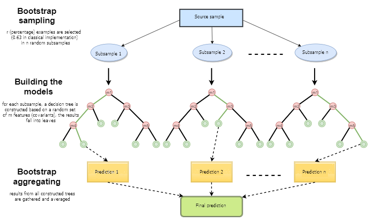
Fig. 1. Scheme of random forest operation

The random forest algorithm proved to be extremely effective, capable of solving practical problems. It provides a high quality of training with a seemingly large number of randomness introduced into the process of constructing the model. The advantage over other machine learning models is an out-of-bag estimate for a part of the set that is not included in the training sample. Therefore, cross-validation or testing on a single sample are not necessary for the decision trees. It suffices to limit ourselves to the out-of-bag estimate for further "tuning" of the model: selecting the number of decision trees and the regularizing component. 

The ALGLIB library, included in the standard МetaТrader 5 package, contains the Random Decision Forest (RDF) algorithm. It is a modification of the original Random Forest algorithm proposed by Leo Breiman and Adele Cutler. This algorithm combines two ideas: using a committee of decision trees which obtains the result by voting and the idea of randomizing the learning process. More details on modifications of the algorithm can be found on the ALGLIB website.

Advantages of the algorithm

• High learning speed
• Non-iterative learning — the algorithm is completed in a fixed number of operations
• Scalability (ability to handle large amounts of data)
• High quality of the obtained models (comparable to neural networks and ensembles of neural networks)
• No sensitivity to spikes in data due to random sampling
• A small number of configurable parameters
• No sensitivity to scaling of feature values (and to any monotonous transformations in general) due to selection of random subspaces
• Does not require careful configuration of parameters, works well out of the box. "Tuning" of parameters allows for an increase in accuracy from 0.5% to 3% depending on the task and data.
• Works well with missing data — retains good accuracy even if a large portion of the data is missing.
• Internal assessment of the model's generalization ability.
• The ability to work with raw data, without preprocessing.

Disadvantages of the algorithm

• The constructed model takes up a large amount of memory. If a committee is constructed from K trees based on a training set of size N, then the memory requirements are O(K·N). For example, for K=100 and N=1000, the model constructed by ALGLIB takes about 1 MB of memory. However, the amount of RAM in modern computers is large enough, so this is not a major flaw.
  
• A trained model works somewhat slower than other algorithms (if there are 100 trees in a model, it is necessary to iterate over all of them to obtain the result). On modern machines, however, this is not so noticeable.
• The algorithm works worse than most linear methods when a set has a lot of sparse features (texts, Bag of words) or when the objects to be classified can be separated linearly.
• The algorithm is prone to overfitting, especially on noisy tasks. Part of this problem can be solved by adjusting the r parameter. A similar, but a more pronounced problem also exists for the original Random Forest algorithm. However, the authors claimed the algorithm is not susceptible to overfitting. This fallacy is shared by some machine learning practitioners and theorists.
• For data that include categorical variables with a different number of levels, random forests are biased in favor of features with more levels. A tree will be more strongly adjusted to such features, as they allow receiving a higher value of optimized functional (type of information gain).
• Similar to the decision trees, the algorithm is absolutely incapable of extrapolation (but this can be considered a plus, since there will be no extreme values in case of a spike)

Peculiarities of the use of machine learning in trading

Among the neophytes of machine learning, there is a popular belief that it is some sort of fairy-tale world, where programs do everything for a trader, while he simply enjoys the profit received. This is only partially true. The end result will depend on how well the problems described below are solved.

• Feature selection

The first and main problem is the choice of what exactly the model needs to be taught. The price is affected by many factors. There is only one scientific approach to studying the market — Econometrics. There are three main methods: regression analysis, time series analysis and panel analysis. A separate interesting section in this field is nonparametric econometrics, which is based solely on available data, without an analysis of the causes that form them. Methods of nonparametric econometrics have recently become popular in the applied research: for example, these include kernel methods and neural networks. The same section includes mathematical analysis of non-numeric concepts — for example, fuzzy sets. If you intend to take machine training seriously, an introduction to econometric methods will be helpful. This article will focus on the fuzzy sets.

• Model selection

The second problem is the choice of the training model. There are many linear and nonlinear models. Their list and comparison of characteristics can be found on the Microsoft site, for instance.

For example, there is a huge variety of neural networks. When using them, you have to experiment with the network architecture, selecting the number of layers and neurons. At the same time, classical MLP-type neural networks are trained slowly (especially gradient descent with a fixed step), experiments with them take a lot of time. Modern fast learning Deep Learning networks are currently unavailable in the standard library of the terminal and including third-party libraries in the DLL form is not very convenient. I have not yet sufficiently studied such packages.

Unlike neural networks, linear models work fast, but do not always handle the approximation well.

Random Forest does not have these drawbacks. It is only necessary to select the number of trees and the parameter r responsible for the percentage of objects that fall into the training sample. Experiments in Microsoft Azure Machine Learning Studio have shown that random forests give the smallest error of prediction on the test data in most cases.

• Model testing

In general, there is only one strict recommendation: the larger the training sample and the more informative the features, the more stable the system should be on the new data. But when solving the tasks of trading, a case of insufficient system capacity may occur, when the mutual variations of the predictors are too few and they are not informative. As a result, the same signal from the predictors will generate both buy and sell signals. The output model will have a low generalizing ability and, as a consequence, poor signal quality in the future. In addition, training on a large sample will be slow, rendering multiple runs during optimization impossible. With all this, there will be no guarantee of a positive result. Add to these problems the chaotic nature of quotes, with their non-stationarity, constantly changing market patterns or (worse) with their complete absence.

Selecting the model training method

Random forest is used to solve a wide range of regression, classification and clustering problems.

These methods can be represented as follows.

• Unsupervised learning. Clustering, detection of anomalies. These methods are applied to programmatically divide features into groups with distinctive differences determined automatically.
• Supervised learning. Classification and regression. A set of previously known training examples (labels) is fed as input, and the random forest tries to learn (approximate) all cases.
• Reinforcement learning. This is perhaps the most unusual and promising kind of machine learning, which stands out from the rest. Here, learning occurs when the virtual agent interacts with the environment, while the agent tries to maximize the rewards received from actions in this environment. Let us use this approach.

Reinforcement learning in Trading System development tasks

Imagine creating a trader with artificial intelligence. It will interact with the environment and receive a certain response to its actions from the environment. For example, profitable trades will be encouraged and it will be fined for unprofitable trades. In the end, after several episodes of interaction with the market, the artificial trader will develop its own unique experience, which will be imprinted on its "brain". The random forest will act as the "brain".

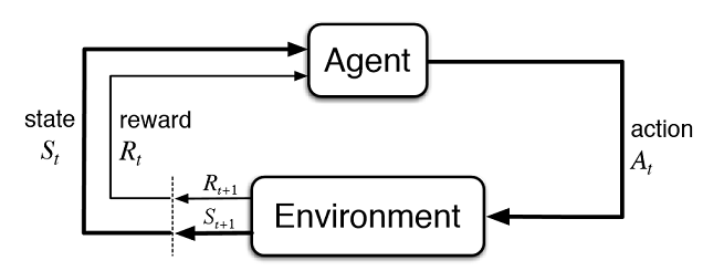
Fig. 2. Interaction of the virtual trader with the market

Figure 2 presents the interaction scheme of the agent (artificial trader) with the environment (market). The agent can perform actions A at time t, while being in state St. After that it goes into state St+1, receiving reward Rt for the previous action from the environment depending on how successful it was. These actions may continue t+n times, until the entire studied sequence (or a game episode for the agent) is complete. This process can be made iterative, making the agent learn multiple times, constantly improving the results.

The agent's memory (or experience) should be stored somewhere. The classic implementation of the reinforced learning uses state-action matrices. When entering a certain state, the agent is forced to address the matrix for the next decision. This implementation is suitable for tasks with a very limited set of states. Otherwise, the matrix can become very large. Therefore, the table is replaced with a random forest:

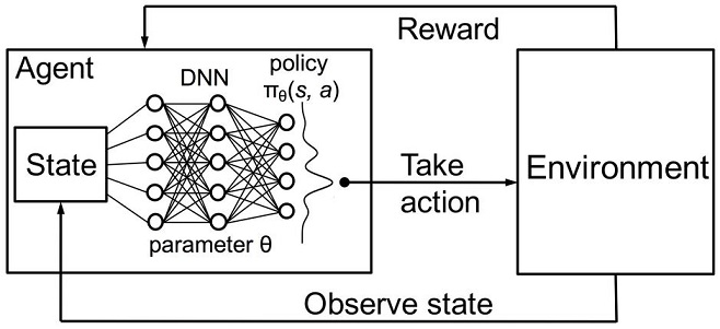
Fig. 3. Deep neural network or random forest for approximation of policy

A stochastic parametrized policy Πθ of an agent is a set of (s,a) pair, where θ is the vector of parameters for each state. The optimal policy is the optimal set of actions for a particular task. Let us agree that the agent seeks to develop an optimal policy. This approach works well for continuous tasks with a previously unknown number of states and is a model-free Actor-Critic method in Reinforcement learning. There are many other approaches to Reinforcement learning. They are described in the "Reinforcement Learning: An Introduction" book by Richard S. Sutton and Andrew G. Barto.

Software implementation of a self-learning expert (agent)

I strive for continuity in my articles, therefore the fuzzy logic system will act as an agent. In the previous article, the Gaussian membership function was optimized for the Mamdani fuzzy inference. However, that approach had a significant disadvantage — the Gaussian remained unchanged for all cases, regardless of the current state of the environment (indicator values). Now the task is to automatically select the position of the Gaussian for the "neutral" term of the fuzzy output "out". The agent will be tasked with development of the optimal policy by selecting values and approximating the function of the Gaussian's center, depending on the values of three values and in the range of [0;1].

Create a separate pointer to the membership function in the global variables of the expert. This allows us to freely change its parameters in the process of learning:

CNormalMembershipFunction *updateNeutral=new CNormalMembershipFunction(0.5,0.2);

Create a random forest and matrix class objects to fill it with values:

//RDF system. Here we create all RF objects.
CDecisionForest      RDF;                                     //Random forest object
CMatrixDouble        RDFpolicyMatrix;                         //Matrix for RF inputs and output
CDFReport            RDF_report;                              //RF return errors in this object, then we can check it

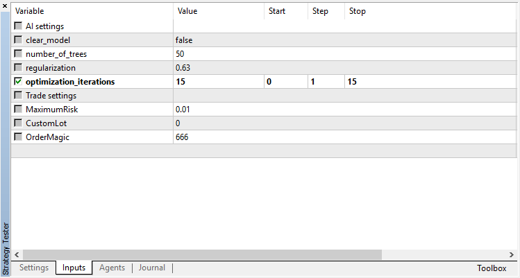
The main settings of the random forest are moved to input parameters: the number of trees and the regularizing component. This allows slightly improving the model by tuning these parameters:

sinput int number_of_trees=50;
sinput double regularization=0.63;

Let us write a service function for checking the state of the model. If the random forest has already been trained for the current timeframe, it will be used for trading signals, and if not — initialize the policy with random values (trade randomly).

void checkBeforeLearn()
  {
   if(clear_model)
     {
      int clearRDF=FileOpen("RDFNtrees"+_Symbol+(string)_Period+".txt",FILE_READ|FILE_WRITE|FILE_CSV|FILE_ANSI|FILE_COMMON);
      FileWrite(clearRDF,0);
      FileClose(clearRDF);
      ExpertRemove();
      return;
     }

   int filehnd=FileOpen("RDFNtrees"+ _Symbol + (string)_Period +".txt",FILE_READ|FILE_WRITE|FILE_CSV|FILE_ANSI|FILE_COMMON);
   int ntrees =  (int)FileReadNumber(filehnd);
   FileClose(filehnd);

   if(ntrees>0)
     {
      random_policy=false;

      int setRDF=FileOpen("RDFBufsize"+_Symbol+(string)_Period+".txt",FILE_READ|FILE_WRITE|FILE_CSV|FILE_ANSI|FILE_COMMON);
      RDF.m_bufsize=(int)FileReadNumber(setRDF);
      FileClose(setRDF);

      setRDF=FileOpen("RDFNclasses"+_Symbol+(string)_Period+".txt",FILE_READ|FILE_WRITE|FILE_CSV|FILE_ANSI|FILE_COMMON);
      RDF.m_nclasses=(int)FileReadNumber(setRDF);
      FileClose(setRDF);

      setRDF=FileOpen("RDFNtrees"+_Symbol+(string)_Period+".txt",FILE_READ|FILE_WRITE|FILE_CSV|FILE_ANSI|FILE_COMMON);
      RDF.m_ntrees=(int)FileReadNumber(setRDF);
      FileClose(setRDF);

      setRDF=FileOpen("RDFNvars"+_Symbol+(string)_Period+".txt",FILE_READ|FILE_WRITE|FILE_CSV|FILE_ANSI|FILE_COMMON);
      RDF.m_nvars=(int)FileReadNumber(setRDF);
      FileClose(setRDF);

      setRDF=FileOpen("RDFMtrees"+_Symbol+(string)_Period+".txt",FILE_READ|FILE_WRITE|FILE_BIN|FILE_ANSI|FILE_COMMON);
      FileReadArray(setRDF,RDF.m_trees);
      FileClose(setRDF);
     }
   else Print("Starting new learn");

   checked_for_learn=true;
  }

As you can see from the listing, the trained model is loaded from files containing:

• the size of the training sample,
  
• the number of classes (1 in case of a regression model),
  
• the number of trees,
  
• the number of features,
• and the array of trained trees.

Training will take place in the strategy tester, in the optimization mode. After each pass in the tester, the model will be trained on the newly formed matrix and stored in the above files for later use:

double OnTester()
  {
   if(clear_model) return 0;

   if(MQLInfoInteger(MQL_OPTIMIZATION)==true)
     {
      if(numberOfsamples>0)
        {
         CDForest::DFBuildRandomDecisionForest(RDFpolicyMatrix,numberOfsamples,3,1,number_of_trees,regularization,RDFinfo,RDF,RDF_report);
        }

      int filehnd=FileOpen("RDFBufsize"+_Symbol+(string)_Period+".txt",FILE_READ|FILE_WRITE|FILE_CSV|FILE_ANSI|FILE_COMMON);
      FileWrite(filehnd,RDF.m_bufsize);
      FileClose(filehnd);

      filehnd=FileOpen("RDFNclasses"+_Symbol+(string)_Period+".txt",FILE_READ|FILE_WRITE|FILE_CSV|FILE_ANSI|FILE_COMMON);
      FileWrite(filehnd,RDF.m_nclasses);
      FileClose(filehnd);

      filehnd=FileOpen("RDFNtrees"+_Symbol+(string)_Period+".txt",FILE_READ|FILE_WRITE|FILE_CSV|FILE_ANSI|FILE_COMMON);
      FileWrite(filehnd,RDF.m_ntrees);
      FileClose(filehnd);

      filehnd=FileOpen("RDFNvars"+_Symbol+(string)_Period+".txt",FILE_READ|FILE_WRITE|FILE_CSV|FILE_ANSI|FILE_COMMON);
      FileWrite(filehnd,RDF.m_nvars);
      FileClose(filehnd);

      filehnd=FileOpen("RDFMtrees"+_Symbol+(string)_Period+".txt",FILE_READ|FILE_WRITE|FILE_BIN|FILE_ANSI|FILE_COMMON);
      FileWriteArray(filehnd,RDF.m_trees);
      FileClose(filehnd);
     }

   return 0;
  }

The function for processing trade signals from the previous article remains practically unchanged, but now the following function is called after opening an order: 

void updatePolicy(double action)
  {
   if(MQLInfoInteger(MQL_OPTIMIZATION)==true)
     {
      numberOfsamples++;
      RDFpolicyMatrix.Resize(numberOfsamples,4);

      RDFpolicyMatrix[numberOfsamples-1].Set(0,arr1[0]);
      RDFpolicyMatrix[numberOfsamples-1].Set(1,arr2[0]);
      RDFpolicyMatrix[numberOfsamples-1].Set(2,arr3[0]);
      RDFpolicyMatrix[numberOfsamples-1].Set(3,action);
     }
  }

It adds a state vector with values of three indicators to the matrix, and the output value is filled with the current signal obtained from the Mamdani fuzzy inference.

Another function:

void updateReward()
  {
   if(MQLInfoInteger(MQL_OPTIMIZATION)==true)
     {
      int unierr;
      if(getLAstProfit()<0) RDFpolicyMatrix[numberOfsamples-1].Set(3,MathRandomUniform(0,1,unierr));
     }
  }

is called every time after an order is closed. If a trade turns out to be unprofitable, then the reward for the agent is selected from a random uniform distribution, otherwise the reward remains unchanged.

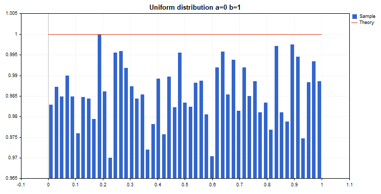
Fig. 4. Uniform distribution for selecting a random reward value

Thus, in the current implementation, the profitable trades made by the agent are encouraged, and in case of unprofitable ones the agent is forced to take a random action (random position of the Gaussian's center) in search of the optimal solution.

The complete code of the signal processing function looks as follows:

void PlaceOrders(double ts)
  {
   if(CountOrders(0)!=0 || CountOrders(1)!=0)
     {
      for(int b=OrdersTotal()-1; b>=0; b--)
         if(OrderSelect(b,SELECT_BY_POS)==true)
            if(OrderSymbol()==_Symbol && OrderMagicNumber()==OrderMagic)

               switch(OrderType())
                 {
                  case OP_BUY:
                     if(ts>=0.5)
                     if(OrderClose(OrderTicket(),OrderLots(),OrderClosePrice(),0,Red))
                       {
                        updateReward();
                        if(ts>0.6)
                          {
                           lots=LotsOptimized();
                           if(OrderSend(Symbol(),OP_SELL,lots,SymbolInfoDouble(_Symbol,SYMBOL_BID),0,0,0,NULL,OrderMagic,Red)>0)
                             {
                              updatePolicy(ts);
                             };
                          }
                       }
                     break;

                  case OP_SELL:
                     if(ts<=0.5)
                     if(OrderClose(OrderTicket(),OrderLots(),OrderClosePrice(),0,Red))
                       {
                        updateReward();
                        if(ts<0.4)
                          {
                           lots=LotsOptimized();
                           if(OrderSend(Symbol(),OP_BUY,lots,SymbolInfoDouble(_Symbol,SYMBOL_ASK),0,0,0,NULL,OrderMagic,Green)>0)
                             {
                              updatePolicy(ts);
                             };
                          }
                       }
                     break;
                 }
      return;
     }

   lots=LotsOptimized();

   if((ts<0.4) && (OrderSend(Symbol(),OP_BUY,lots,SymbolInfoDouble(_Symbol,SYMBOL_ASK),0,0,0,NULL,OrderMagic,INT_MIN) > 0))
      updatePolicy(ts);
   else if((ts>0.6) && (OrderSend(Symbol(),OP_SELL,lots,SymbolInfoDouble(_Symbol,SYMBOL_BID),0,0,0,NULL,OrderMagic,INT_MIN) > 0))
      updatePolicy(ts);
   return;
  }

The function for calculating the Mamdani fuzzy inference has undergone changes. Now, if the agent's policy was not selected randomly, it calls the calculation of the Gaussian's position along the X axis using the trained random forest. The random forest is fed the current state as a vector with 3 oscillator values, and the obtained result updates the position of the Gaussian. If the EA is run in the optimizer for the first time, the position of the Gaussian is selected randomly for each state.

double CalculateMamdani()
  {
   CopyBuffer(hnd1,0,0,1,arr1);
   NormalizeArrays(arr1);

   CopyBuffer(hnd2,0,0,1,arr2);
   NormalizeArrays(arr2);

   CopyBuffer(hnd3,0,0,1,arr3);
   NormalizeArrays(arr3);

   if(!random_policy)
     {
      vector[0]=arr1[0];
      vector[1]=arr2[0];
      vector[2]=arr3[0];

      CDForest::DFProcess(RDF,vector,RFout);
      updateNeutral.B(RFout[0]);
     }
   else
     {
      int unierr;
      updateNeutral.B(MathRandomUniform(0,1,unierr));
     }
   
   //Print(updateNeutral.B());
   firstTerm.SetAll(firstInput,arr1[0]);
   secondTerm.SetAll(secondInput,arr2[0]);
   thirdTerm.SetAll(thirdInput,arr3[0]);

   Inputs.Clear();
   Inputs.Add(firstTerm);
   Inputs.Add(secondTerm);
   Inputs.Add(thirdTerm);

   CList *FuzzResult=OurFuzzy.Calculate(Inputs);
   Output=FuzzResult.GetNodeAtIndex(0);
   double res=Output.Value();
   delete FuzzResult;

   return(res);
  }

The process of training and testing the model

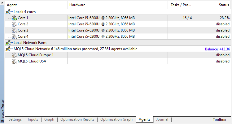
The agent will be trained in the optimizer sequentially. That is, the results of the previous training written to files will be used for the next run. To do this, simply disable all testing agents and the cloud, leaving only one core. 

Disable the genetic algorithm (use slow complete algorithm). Training/testing is performed using Open prices, because the EA explicitly controls new bar opening.

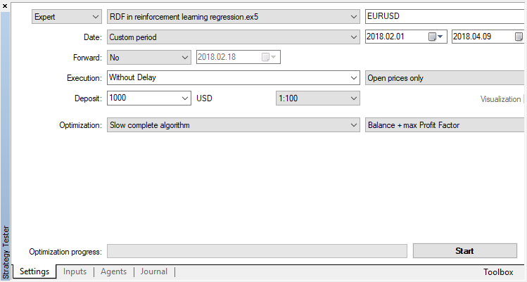
There is only one optimizable parameter — the number of passes in the optimizer. To demonstrate the algorithm operation, set 15 iterations.

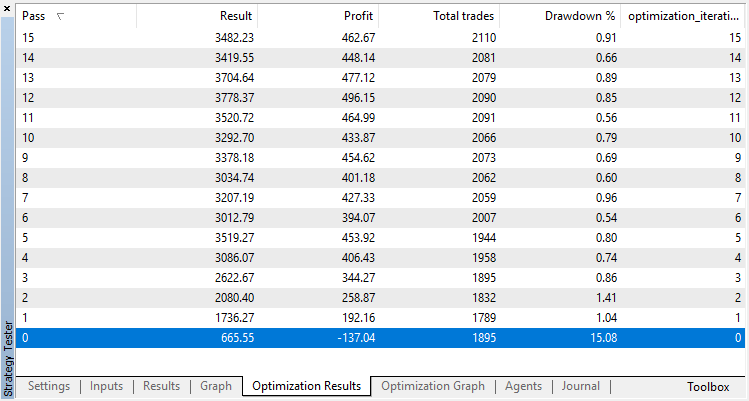
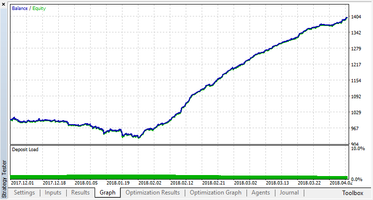
Optimization results of the regression model (with one output variable) are presented below. Keep in mind that the trained model is saved to a file, so only the result of the last run will be saved.

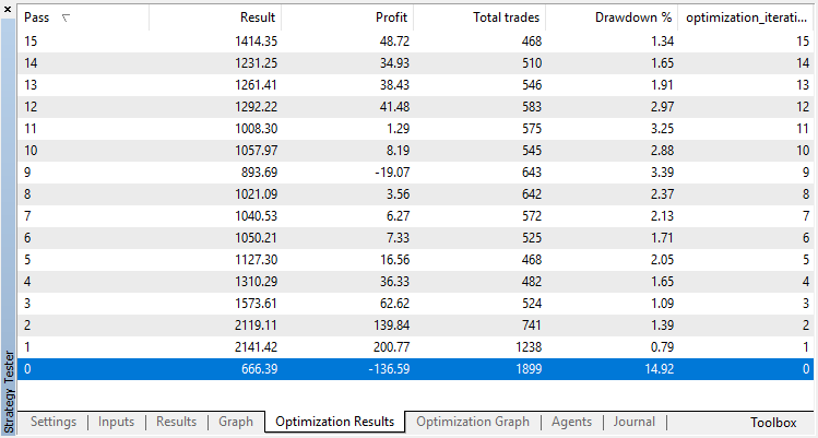
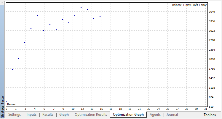
The zero run corresponds to the random policy of the Agent (first run), so it caused the largest loss. The first run, on the contrary, turned out to be the most productive. Subsequent games did not give a gain, but stagnated. As a result, the growth chart looks as follows after the 15th run:

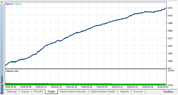
Let us carry out the same experiment for the classification model. In this case, the rewards are divided into 2 classes — positive and negative.

Classification performs this task much better. At least there is a stable growth from the zero run, corresponding to the random policy, up to the 15th, where the growth stopped and the policy started fluctuating about around the optimum.

The final result of the Agent's training:

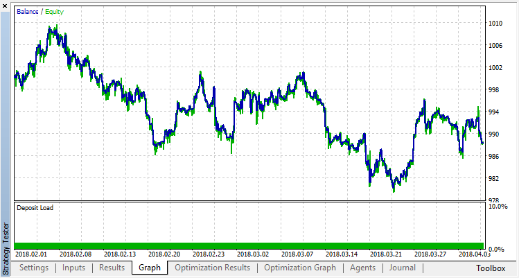
Check the results of the system operation on a sample outside the training range. The model was greatly overfitted:

Let us try to get rid of overfitting. Set the parameter r (regularization) to 0.25: only 25% of the sample will be used in training. Use the same training range.

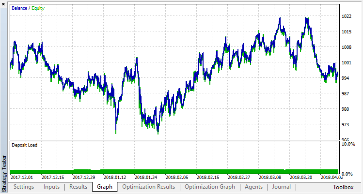
The model has learned worse (more noise is added), but it was not possible to get rid of global overfitting. This regularization method is obviously suitable only for stationary processes in which the regularities do not change over time. Another obvious negative factor is the 3 oscillators at the input of the model, which, in addition, correlate with each other.

Summing up the article

The objective was to show the possibilities of using a random forest to approximate a function. In this case, the function of indicator values was a buy or sell signal. Also, two types of supervised learning were considered — classification and regression. A nonstandard approach was applied to learning with previously unknown training examples that were selected automatically during the optimization process. In general, the process is similar to a conventional optimization in the tester (cloud), with the algorithm converging in just a few iterations and without the need to worry about the number of optimized parameters. That is a clear advantage of the applied approach. Disadvantage of the model is a strong tendency of overfitting when the strategy is selected incorrectly, which is equivalent to over-optimization of the parameters. 

By tradition, I will give possible ways to improve the strategy (after all, the current implementation is only a rough frame).

• Increasing the number of optimized parameters (optimization of multiple membership functions).
• Adding various significant predictors.
• Applying different methods of rewarding the agent.
• Creating several rival agents to increase the space of variants.

The source files of the self-learning expert are attached below.

For the expert to work and compile, it is necessary to download the MT4Orders library and the updated Fuzzy library.