Risk Evaluation in the Sequence of Deals with One Asset
Aleksey Nikolayev | 16 October, 2017
Foreword
In this article, we will draw on the idea of Ralph Vince on managing position volumes (in this connection, it will be useful to recall the Kelly formula as well). This is also known as the optimal f. In this theory, f is the fraction of funds that is at risk in every deal. According to Vince, f is chosen depending on the conditions of optimization (maximization) of profit. There are two problems arising when using this theory in trading. They are:
- Too large account drawdown.
- f is known only on the history of deals.
An attempt to solve these problems is only one of the aims of this article. Another problem is yet another attempt to introduce the theory of probability and mathematical statistics into the analysis of trading systems. This will cause occasional deviation from the main topic. I will refrain from expounding the basics. If the necessity arises, the reader can refer to the book "The Mathematics of Technical Analysis: Applying Statistics to Trading Stocks, Options and Futures".
This article features examples. They are just an illustration of the theory considered in the article, therefore, they are not recommended to be used in real trading.
Introduction. Absence of uncertainty
For the sake of simplicity, let us assume that the price of an asset expresses the value of its unit in the units of capital and not the other way round. Minimal volume step is a fixed value in the units of asset. Minimal non-zero volume of the deal is equal to this step. We will use a simple deal model.
For each deal defined are its type (buy/sell), its volume v along with the prices of entry, stop loss and exit penter, pstop and pexit accordingly.
Obvious contraints:
- non-zero volume v≥0
- the stop price must be lower than the entry price when buying: pstop<penter
- the stop price must be greater than the entry price when selling : pstop>penter.
Let us introduce the following notations:
- C0 — capital before entering the deal;
- C1 — capital after exiting the deal;
- Cs — capital after stop loss is triggered;
- r — the share of the initial capital lost when stop loss is triggered,
that is C0−Cs=rC0.
For the deal of the buy type: C1=C0+v(pexit−penter) and Cs=C0−v(penter−pstop).
Same for the deal of the sell type: C1=C0+v(penter−pexit) and Cs=C0−v(pstop−penter).
After simple rearrangements we will arrive at C1=C0(1+ra) where a=(pexit−penter)/(penter−pstop). These expressions are true for deals of both buy and sell types. Let us call the r value the risk of the deal and the a value the yield on the deal.
Let us state the problem of managing risks for our model. Let us assume that we have n deals with the yields ai where i=1..n,. We want to estimate risks ri. It should be taken into account that ri can only depend on the values known when entering the deal. Risks are usually considered to be equal to each other ri=r where 0≤r<1. r=rmax is the value that maximizes the profit Cn=C0(1+ra1)(1+ra2)…(1+ran).
We will have a similar approach with some differences. We will take into account some contraints. These are the maximum drawdown and the average yield in a series of deals. Let us introduce the following notations:
- A0 is the least of all ai,
- A=(a1+a2+…+an)/n is their arithmetic average.
It is always true that A0≤A and the equality is achieved only when all ai=A0. Let us consider contraints to r in more detail.
- Cn=Cn(r)>0 whence it follows that 1+rA0>0. If A0≥−1 then this is true for all 0≤r<1. In case when A0<−1 we receive 0≤r<−1/A0. We can see that an additional restriction to r appears only when there are deals exited by stop loss with slippage. As a result, the restriction will be written as 0≤r<rc where rc=1, if A0≥−1 and rc=−1/A0 if A0<−1.
-
We will define the average yield g as Cn=C0(1+gr)^n hence

In other words, g can be called the average yield of the deal in a series in relation to accepted risk. The g(r) function is defined during carrying out contraint of the previous point. It has a removable singularity in the point r=0: if r→0 then g(r)→A and we can accept that g(0)=A. It may be shown that g(r)≡A only if all ai=A. If amongst ai there are different ones then g(r) decreasing when r is increasing. The restriction will look like g(r)≥G0>0. The constant G0 depends on many things - conditions of trade, the trader's preferences etc. In current model, it can be said that if G0>A, then a set of r satisfying the inequality will be empty. If G0≤A, then our restriction will look like 0≤r≤rg where rg is the solution of the equation g(rg)=G0. If this equation does not have solutions, then rg=1.
-
To evaluate maximum drawdown, let us consider its opposite value:

This value can be called the minimal gain. It is convenient as it is always positive and finite when the restriction specified in the first point is met. It is evident that d(0)=1. If A0<0, then d(r) is decreasing when r is increasing in the area limited by the first point. The restriction will be written as d(r)≥D0 where 0<D0<1. The greater D0, the smaller the drawdown is permitted. Let us rewrite our restriction as 0≤r≤rd where rd is the solution of the equation d(rd)=D0 (if this equation does not have solutions, then rd=1).
-
When the deal is entered, the volume v cannot have an arbitrary value. It has to be divisible by some value Δv>0 that is v=kΔv where integer k≥0. Then, for the ith deal:

Apparently, coincidence of all ri is highly unlikely. Consequently, the problem stated above does not have a precise solution. We will look for an approximate solution. We will confine ourselves to calculating such a minimal rv so that ri can take at least one non-zero value inside [0,rv].

Let us also determine a rough evaluation rvr≥rv. From fulfilling the restriction in the previous point it follows that Ci≥D0C0>0. Whence it follows that (please note that d0 and D0 mean the same thing):

This evaluation is convenient because it has a more simple relationship with the capital. It depends only on the initial value of the capital.
We assume that the set satisfying the first three contraint is not empty. Then it will look like the interval [0,ra] where ra=min(rc,rg,rd).
We also assume also that the fourth restriction is met too. This requires that ra≥rv. We are going to consider a problem of maximization Cn=Cn(r). In a significant case, A>0 and A0<0. This function is increasing on the interval [0,rmax] and decreasing on the interval [rmax,rc]. Here rmax is the stationary point of the first order derivative dCn(r)/dr=0.
We can easily find ropt which maximizes Cn(r) on the interval [0,ra]: ropt=min(ra,rmax). There are two cases remaining: 1) A0≤A≤0 and 2) 0≤A0≤A. In the first case, ropt=rmax=0, and in the second case rmax=rс and ropt=ra .
Now, we are going to consider the case when the set defined by contraint, is empty. This is possible only in two cases: 1) G0>A or 2) ra<rv. We only have to assume that ropt=0.
Now, we are going to find values ri taking into account the discrete nature of the deal volumes. Let Ri be a non-empty finite set of numbers on the interval [0,ra] suitable for the value of risk ri in the ith deal. Select ropt,i which maximizes Cn(r) on Ri. If ropt∈Ri then ropt,i=ropt. If ropt∉Ri, then two situations are possible: 1) all points Ri belong to one side from ropt and 2) points Ri belong to two sides from ropt. In the first case, ropt,i will be a point from Ri closest to ropt. In the second case, Ri will be two points closest to the ropt on each side. The ropt,i will be the point in which Cn(r) is greater.
Uncertainty. Introductory example
Let us make the model considered in the introduction more complex. Let us assume that we know n numbers of ai but we do not know their order. This way, their random permutation is allowed. Let us see what will change in the results obtained above. In the first two points, the random permutation of ai will not change anything. There will not be any changes in the forth point if a more rough evaluation rvr is used.
Changes are possible in the third point. Indeed, if the sequence is arranged in the way so there are no positive values between negative ones, then the drawdown will be maximum. Conversely, evenly mixed positive and negative numbers will reduce the drawdown. The total number of permutations in the general case equals to n!. This is a very large number with n being in the range of several tens. In theory, we can solve the problem set in the introduction for each of j=1..n! permutations from the sequence ai and obtain a set of numbers rd,j. There is, however, a persisting issue. We do not know what permutation to select. To work with this uncertainty, we need to deploy the concepts and methods of the theory of probabilities and mathematical statistics.
Let us consider a set of numbers rd,j as values of the ρd=ρd(j)=rd,j function that depends on the permutation. In terms of the theory of probabilities, ρd is a random variable for which a set of elementary events equals to a set of n permutations. We will treat them all as different even if some ai are the same.
We also assume that all n permutations are equally likely. Then the probability of each of them is 1/n!. This defies the probabilistic measure on the set of elementary events. Now, we can define the distribution of probabilities ρρd(x)=n(x)/n! for Pd where n(x) is the number of n permutations for which rd,j<x. At this point, the restriction qualification for the drawdown must be specified. Along with minimal permitted D0, we must specify acceptable significance level 0<δ<<1. δ indicates what probability of exceeding the threshold drawdown we consider negligible. Then, we can define rd(δ) as the δ quantile of the distribution Pρd(x). To find an approximate solution to this problem, we are going to randomly generate a large number of nt, where 1<<nt<<n!, n permutations. Let us find the value rd,j for each of them, where 1≤j≤nt. Then, for evaluation for rd(δ), we can take a sample δ quantile of the rd,j population.
Although this model is slightly artificial, it has its uses. For instance, we can take rd, calculated for the initial series of deals and find the probability pd=Pρd(rd). Obviously, the 0≤pd≤1 inequality is valid. pd close to zero indicates a large drawdown caused by loss-making deals gathered close to each other. A pd close to one shows that profitable and loss-making deals were uniformly mixed. This is the way not only to discover a series of losses in a sequence of deals (for instance, like in the Z-score method) but also a degree of its influence on the drawdown. Other indices depending either on Pρd() or on rd can be generated.
Uncertainty. General case
Let us assume that there is a sequence of deals with yields ai, 1≤i≤n. We will also assume that this sequence is an implementation of a sequence of independent in a population and identically distributed random variables λi. Let us write their probability distribution function as Pλ(x). It is supposed that it has the following properties:
- positive mathematical expectation Mλ
- limitation from below. There is a number λmin≤−1 for which Pλ(x)=0 when x<λmin and Pλ(x)>0 when x>λ0.
These conditions mean that the average yield is positive. Although, loss-making deals are probable, there is always a possibility not to loose all capital in one deal by limiting the risk.
Let us state the problem of identifying the magnitude of the risk. Similar to the example in the previous part, we should study a random variable ρopt instead of ropt calculated in the introduction. Then, having set the significance level δ, let us calculate ropt=ropt(δ) where δ is a quantile of the Pρopt(x) distribution. This system with this risk can be used until the drawdown and the average yield are in the set range. When they exceed the range boundaries, this system should be discarded. The probability of error will not exceed δ.
The importance of smallness of δ should be emphasized. Using the obtained criterion does not make any sense when δ if great. Only in case of small δ two events can be believe to be connected with each other: 1) the system does not work due to the changes on the market and 2) either the drawdown is too great or the yield is too small. Along with the error that has already been discussed, another error can be considered. When that error is present, we do not notice market changes that affect the drawdown and the yield of our system. There is not point to discuss this error as it does not affect the yield of the system.
In our theory, it manifests in the fact that the changes of the Pλ(x) and Pρopt(x) distributions are not important for us. The only thing that matters is the change of the δ quantile Pρopt(x). Particularly, this means that there is no stationarity requirement to the sequence of yields. Saying that, we will need stationarity for restoring the law of yield distribution on the final sample ai, 1≤i≤n. Here, the requirement that the distribution does not change significantly may be sufficient instead of absolute stationarity.
In the end, ρopt can be expressed through λi, though this is a complex relationship (it is expressed though other random intermediary variables). This calls for studying random variables defined as functions of λi and build their distributions. For that, we need to know Pλ(x). Let us list three variants of what information about this distribution we can have.
- There is an exact expression for Pλ(x) or there is a way to make an arbitrarily close approximation for the trading system under analysis. Usually, this is possible only when there is a founded assumption about the behavior of the asset prices. For instance, we can consider the random walk hypothesis to be true. Using this information in trading is hardly possible. Conclusions drawn this way are unrealistic and usually deny the possibility of profit all together. This can be used differently. Using this hypothesis, we can build the null hypothesis. Then, using empirical data and tests for concordance, we can either discard the hypothesis or admit that we can not discard it with our data. In our case, such empirical data is the sequence ai, 1≤i≤n.
- Pλ(x) is known to belong or coming close to some parametric family of distributions. This is possible when the assumptions about the asset prices from the previous point are not far off. Of course, the type of the distribution family is defined also by the algorithm of the trading system. Exact values for distribution parameters are calculated using the sequence ai, 1≤i≤n by the methods of parametric statistics.
- Along with the sequence ai, 1≤i≤n some common properties of Pλ(x) are known (or assumed). Foe example, this may be a supposition about existing finite expectation and variance. In such case, we will use a sample distribution function as the approximation for Pλ(x). We will build it based on the same sequence ai, 1≤i≤n. Methods using the sample distribution function instead of the exact one are called bootstrap. In some cases, it is not necessary to know Pλ(x). For instance, the random variable (λ1+λ2+…+λn)/n when n are great can be treated as distributed normally (with finite variance λi).
This article will have a continuation where suppositions described in the third variant will be used. The first two variants will be described further.
We will study how the calculations carried out in the introduction will change. Instead of absolute numbers A0 and A, we will deal with random variables expressed through λi the same way: Λ0=min(λ1, λ2, …, λn) and Λ=(λ1+λ2+…+λn)/n.
Let us look at their asymptotic behavior at unrestrictedly growing n. In such a case, it is always true that Λ0→λmin. Let us assume that λi has a finite variance Dλ. Then Λ→Mλ. As mentioned above, we can consider with high accuracy that Λ is normally distributed with expectation Mλ and variance Dλ/n. If exact values of Mλ and Dλ are unknown, then their sample analogs calculated by ai can be used. Empiric distributions for Λ0 and Λ can be also built using bootstrap.
Before calculating ropt(δ) by the bootstrap method, we should take into account the following points about how the calculations carried out in the introduction will change:
- In the first point, due to the asymptotic behavior of Λ0 the evaluation can be roughened to the value rc=−1/λmin. For the sampling distribution, λmin coincides with А0 and, therefore, everything in this point stays the same.
- It is important to make sure that the condition G0≤Λ is broken with probability not greater than δ. For that, the δ quantile of Λ must be no smaller than G0. For the approximate calculation of this quantile, we will use the normal approximation of the distribution Λ. As a result, we will obtain nmin — the estimation from below of the number of deals required for analysis. The standard bootstrap method can be adjusted and sets of samples of growing length can be built for finding nmin. From a theoretical point of view, we will have more or less the same as for the approximation by the normal distribution.
- In the forth point, same as before, we will take a rougher evaluation of rvr.
Let us set nb — the number of yield sequences which will be generated. In the cycle of carrying out the bootstrap, we are to iterate over the limitations for the magnitude of the risk for each j=1..nb. Considering the points above, we only have to calculate rg(j), rd(j), rmax(j) and ropt(j). If the set for r at some j is empty, then assume that ropt(j)=0.
At the end of bootstrap, we will have an array of values ropt[]. Having calculated by this array the sample δ quantile, treat it as the solution to the set problem.Conclusion
Everything written above is just the beginning of the theme. I am going to briefly mention what the following articles will be dedicated to.
- To use the deal model as a sequence of independent distributions, we should make some assumptions and suppositions about the asset prices and the trading algorithm.
- This theory must be made more specific for some particular methods of exiting the deal such as fixed stop-loss/take-profit and fixed trailing stop.
- It is also necessary to show how this theory can be used for building trading systems. We will consider how the probability theory can be used for building a system on gaps. We will also touch on the use of machine learning.
Appendix to the introduction
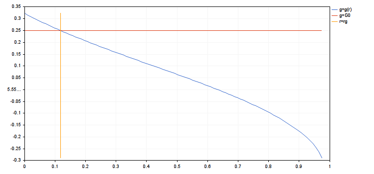
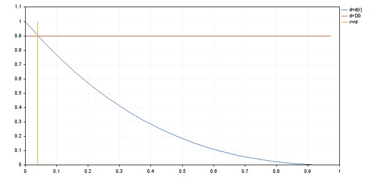
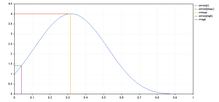
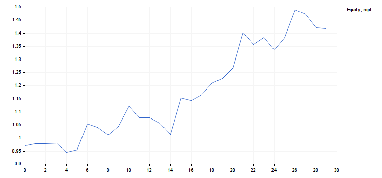
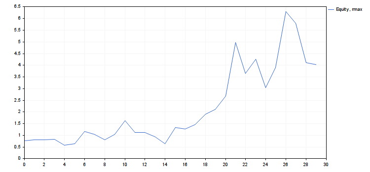
Below is the text of the r_intro.mq5 script and the result of its work in charts and numerical results
#include <Graphics\Graphic.mqh>
#define N 30
#define NR 100
#property script_show_inputs
input int ngr=0;    // number of chart displayed
double G0=0.25;     // lowest average yield
double D0=0.9;      // lowest minimal gain
                    // the initial capital c0 is assumed to equal to 1


void OnStart()
  {
   double A0,A,rc,rg,rd,ra,rmax,ropt,r[NR],g[NR],d[NR],cn[NR],a[N]=
     {
      -0.7615,0.2139,0.0003,0.04576,-0.9081,0.2969, // deal yields
      2.6360,-0.3689,-0.6934,0.8549,1.8484,-0.9745,
      -0.0325,-0.5037,-1.0163,3.4825,-0.1873,0.4850,
      0.9643,0.3734,0.8480,2.6887,-0.8462,0.5375,
      -0.9141,0.9065,1.9506,-0.2472,-0.9218,-0.0775
     };
   A0=a[ArrayMinimum(a)];
   A=0; for(int i=0; i<N;++i) A+=a[i]; A/=N;
   rc=1; if(A0<-1) rc=-1/A0;
   double c[N];
   r[0]=0; cn[0]=1; g[0]=A; d[0]=1;
   for(int i=1; i<NR;++i)
     {
      r[i]=i*rc/NR;
      cn[i]=1; for(int j=0; j<N;++j) cn[i]*=1+r[i]*a[j];
      g[i]=(MathPow(cn[i],1.0/N)-1)/r[i];
      c[0]=1+r[i]*a[0]; for(int j=1; j<N;++j) c[j]=c[j-1]*(1+r[i]*a[j]); d[i]=dcalc(c);
     }
   int nrg,nrd,nra,nrmax,nropt;
   double b[NR];
   for(int i=0; i<NR;++i) b[i]=MathAbs(g[i]-G0);
   nrg=ArrayMinimum(b); rg=r[nrg];
   for(int i=0; i<NR;++i) b[i]=MathAbs(d[i]-D0);
   nrd=ArrayMinimum(b); rd=r[nrd];
   nra=MathMin(nrg,nrd); ra=r[nra];
   nrmax=ArrayMaximum(cn); rmax=r[nrmax];
   nropt=MathMin(nra,nrmax); ropt=r[nropt];
   Print("rc = ",rc,"\nrg = ",rg,"\nrd = ",rd,"\nra = ",ra,"\nrmax = ",rmax,"\nropt = ",ropt,
         "\ng(rmax) = ",g[nrmax],", g(ropt) = ",g[nropt],
         "\nd(rmax) = ",d[nrmax],", d(ropt) = ",d[nropt],
         "\ncn(rmax) = ",cn[nrmax],", cn(ropt) = ",cn[nropt]);
   if(ngr<1 || ngr>5) return;
   ChartSetInteger(0,CHART_SHOW,false);
   CGraphic graphic;
   graphic.Create(0,"G",0,0,0,750,350);
   double x[2],y[2];
   switch(ngr)
     {
      case 1: graphic.CurveAdd(r,g,CURVE_LINES,"g=g(r)");
      x[0]=0; x[1]=r[NR-1]; y[0]=G0; y[1]=G0;
      graphic.CurveAdd(x,y,CURVE_LINES,"g=G0");
      x[0]=rg; x[1]=rg; y[0]=g[0]; y[1]=g[NR-1];
      graphic.CurveAdd(x,y,CURVE_LINES,"r=rg");
      break;
      case 2: graphic.CurveAdd(r,d,CURVE_LINES,"d=d(r)");
      x[0]=0; x[1]=r[NR-1]; y[0]=D0; y[1]=D0;
      graphic.CurveAdd(x,y,CURVE_LINES,"d=D0");
      x[0]=rd; x[1]=rd; y[0]=d[0]; y[1]=d[NR-1];
      graphic.CurveAdd(x,y,CURVE_LINES,"r=rd");
      break;
      case 3: graphic.CurveAdd(r,cn,CURVE_LINES,"cn=cn(r)");
      x[0]=0; x[1]=rmax; y[0]=cn[nrmax]; y[1]=cn[nrmax];
      graphic.CurveAdd(x,y,CURVE_LINES,"cn=cn(rmax)");
      x[0]=rmax; x[1]=rmax; y[0]=cn[NR-1]; y[1]=cn[nrmax];
      graphic.CurveAdd(x,y,CURVE_LINES,"r=rmax");
      x[0]=0; x[1]=ropt; y[0]=cn[nropt]; y[1]=cn[nropt];
      graphic.CurveAdd(x,y,CURVE_LINES,"cn=cn(ropt)");
      x[0]=ropt; x[1]=ropt; y[0]=cn[NR-1]; y[1]=cn[nropt];
      graphic.CurveAdd(x,y,CURVE_LINES,"r=ropt");
      break;
      case 4: c[0]=1+ropt*a[0]; for(int j=1; j<N;++j) c[j]=c[j-1]*(1+ropt*a[j]);
      graphic.CurveAdd(c,CURVE_LINES,"Equity, ropt");
      break;
      case 5: c[0]=1+rmax*a[0]; for(int j=1; j<N;++j) c[j]=c[j-1]*(1+rmax*a[j]);
      graphic.CurveAdd(c,CURVE_LINES,"Equity, rmax");
      break;
     }
   graphic.CurvePlotAll();
   graphic.Update();
   Sleep(30000);
   ChartSetInteger(0,CHART_SHOW,true);
   graphic.Destroy();
  }

// the dcalc() function accepts the array of c1, c2, ... cN values and
// returns the minimal gain d. Assume that c0==1
double dcalc(double &c[])
  {
   if(c[0]<=0) return 0;
   double d=c[0], mx=c[0], mn=c[0];
   for(int i=1; i<N;++i)
     {
      if(c[i]<=0) return 0;
      if(c[i]<mn) {mn=c[i]; d=MathMin(d,mn/mx);}
      else {if(c[i]>mx) mx=mn=c[i];}
     }
   return d;
  }
- rc = 0.9839614287119945
- rg = 0.1180753714454393
- rd = 0.03935845714847978
- ra = 0.03935845714847978
- rmax = 0.3148676571878383
- ropt = 0.03935845714847978
- g(rmax) = 0.1507064833125653, g(ropt) = 0.2967587621877231
- d(rmax) = 0.3925358395456308, d(ropt) = 0.9037200051227304
- cn(rmax) = 4.018198063206267, cn(ropt) = 1.416754202013712
- Use ropt as the risk value in this system.
- The risk freed at this rmax−ropt can be used for adding new systems (diversification).
Appendix to the introductory example
Below is the text of the r_exmp.mq5 script and numerical results of its work.
#include <Math\Stat\Uniform.mqh>
#define N 30      // length of deal series
#define NR 500    // number of segments the interval is split into  [0,rc]
#define NT 500    // number of generated permutations
double D0=0.9;    // smallest minimal gain
double dlt=0.05;  // significance level

void OnStart()
  {
   double A0,rc,r[NR],d[NR],rd[NT],a[N]=//A,rg,ra,rmax,ropt,g[NR],cn[NR],
     {
      -0.7615,0.2139,0.0003,0.04576,-0.9081,0.2969,// deal yields
      2.6360,-0.3689,-0.6934,0.8549,1.8484,-0.9745,
      -0.0325,-0.5037,-1.0163,3.4825,-0.1873,0.4850,
      0.9643,0.3734,0.8480,2.6887,-0.8462,0.5375,
      -0.9141,0.9065,1.9506,-0.2472,-0.9218,-0.0775
     };
   A0=a[ArrayMinimum(a)];
   rc=1; if(A0<-1) rc=-1/A0;
   for(int i=0; i<NR;++i) r[i]=i*rc/NR;
   double b[NR],c[N];
   int nrd;
   MathSrand(GetTickCount());
   for(int j=0; j<NT;++j)
     {
      trps(a,N);
      for(int i=1; i<NR;++i)
        {
         c[0]=1+r[i]*a[0];
         for(int k=1; k<N;++k) c[k]=c[k-1]*(1+r[i]*a[k]);
         d[i]=dcalc(c);
        }
      for(int i=0; i<NR;++i) b[i]=MathAbs(d[i]-D0);
      nrd=ArrayMinimum(b); rd[j]=r[nrd];
     }
   double p[1],q[1]; p[0]=dlt;
   if(!MathQuantile(rd,p,q)) {Print("MathQuantile() error"); return;}
   PrintFormat("sample %f-quantile rd[] equals %f",p[0],q[0]);
   double rd0=0.03935845714847978;   // value of rd obtained in the introduction
   double pd0=0;                     // correspondent value of pd
   for(int j=0; j<NT;++j) if(rd[j]<rd0) ++pd0; pd0/=NT;
   PrintFormat("for rd = %f value pd = %f",rd0,pd0);
  }
// the dcalc() function accepts the array of c1, c2, ... cN values and
// returns the minimal gain d. Assume that c0==1
double dcalc(double &c[])
  {
   if(c[0]<=0) return 0;
   double d=c[0], mx=c[0], mn=c[0];
   for(int i=1; i<N;++i)
     {
      if(c[i]<=0) return 0;
      if(c[i]<mn) {mn=c[i]; d=MathMin(d,mn/mx);}
      else {if(c[i]>mx) mx=mn=c[i];}
     }
   return d;
  }
// random permutation of the first no greater than min(n,ArraySize(b))
// elements of the b[] array
// the library MathSample() can be used instead of trps()
void trps(double &b[],int n)
  {
   if(n<=1) return;
   int sz=ArraySize(b);
   if(sz<=1) return;
   if(sz<n) n=sz;
   int ner;
   double dnc=MathRandomUniform(0,n,ner);
   if(!MathIsValidNumber(dnc)) {Print("Error ",ner); ExpertRemove();}
   int nc=(int)dnc;
   if(nc>=0 && nc<n-1)
     { double tmp=b[n-1]; b[n-1]=b[nc]; b[nc]=tmp;}
   trps(b,n-1);
  }
- the sample 0.05 quantile rd[] equals to 0.021647
- for rd = 0.039358 pd = 0.584
The first line of results tells us that we must half the risk in comparison with the result obtained in the introduction. In this case, if the drawdown exceeds the goal (10%) it will mean that the system is likely to have flaws and it should not be used for trading. The error probability (working system is rejected) in this case will be δ (0.05 or 5%). The second line of the result says that the drawdown in the initial series of deals is smaller that it could be on average. It should be noted that 30 deals may be insufficient for evaluating this system. Therefore, it would be useful to carry out detailed analysis of a larger number of deals and see how this affects the results.
Appendix to the general case
Below is the r_cmn.mq5 script where we are trying to evaluate from below the nmin value and the results of the work of the script:
#include <Math\Stat\Normal.mqh>
#include <Math\Stat\Uniform.mqh>
#include <Graphics\Graphic.mqh>
#define N 30        // length of the deal series
#define NB 10000    // number of generated samples for bootstrap
double G0=0.25;     // lowest average yield
double dlt=0.05;    // significance level

void OnStart()
  {
   double a[N]=
     {
      -0.7615,0.2139,0.0003,0.04576,-0.9081,0.2969,   // deal yields
      2.6360,-0.3689,-0.6934,0.8549,1.8484,-0.9745,
      -0.0325,-0.5037,-1.0163,3.4825,-0.1873,0.4850,
      0.9643,0.3734,0.8480,2.6887,-0.8462,0.5375,
      -0.9141,0.9065,1.9506,-0.2472,-0.9218,-0.0775
     };
   double A=MathMean(a);
   double S2=MathVariance(a);
   double Sk=MathSkewness(a);
   double Md=MathMedian(a);
   Print("sample distribution parameters:");
   PrintFormat("average: %f, variance: %f, asymmetry: %f, median: %f",A,S2,Sk,Md);
   PrintFormat("number of deals: %d, dlt value??: %f, G0value??: %f",N,dlt,G0);
// approximation by normal distribution
   Print("approximation by normal distribution:");
   double q0, p0;
   int ner;
   q0=MathQuantileNormal(dlt,A,MathSqrt(S2/N),ner);
   if(!MathIsValidNumber(q0)) {Print("Error ",ner); return;}
   Print("dlt quantile: ",q0);
   p0=MathCumulativeDistributionNormal(G0,A,MathSqrt(S2/N),ner);
   if(!MathIsValidNumber(p0)) {Print("MathIsValidNumber(p0) error ",ner); return;}
   Print("level of significance for G0: ",p0);
// bootstrap
   MathSrand(GetTickCount());
   double b[N],s[NB];
   p0=0;
   for(int i=0;i<NB;++i)
     {
      sample(a,b);
      s[i]=MathMean(b);
      if(s[i]<G0) ++p0;
     }
   p0/=NB;
   double p[1],q[1];
   p[0]=dlt;
   if(!MathQuantile(s,p,q)) {Print("MathQuantile() error"); return;}
   Print("approximation by bootstrap");
   Print("dlt quantile: ",q[0]);
   Print("level of significance for G0: ",p0);
// approximation nmin (approximation by normal distribution)
   int nmin;
   for(nmin=1; nmin<1000;++nmin)
     {
      q0=MathQuantileNormal(dlt,A,MathSqrt(S2/nmin),ner);
      if(!MathIsValidNumber(q0)) {Print("Error ",ner); return;}
      if(q0>G0) break;
     }
   Print("Minimal number of deals nmin (approximation by normal distribution):");
   PrintFormat("no less than %d, value of the dlt quantile: %f",nmin,q0);
  }

void sample(double &a[],double &b[])
  {
   int ner;
   double dnc;
   for(int i=0; i<N;++i)
     {
      dnc=MathRandomUniform(0,N,ner);
      if(!MathIsValidNumber(dnc)) {Print("MathIsValidNumber(dnc) error ",ner); ExpertRemove();}
      int nc=(int)dnc;
      if(nc==N) nc=N-1;
      b[i]=a[nc];
     }
  }
Sample distribution parameters:
- average: 0.322655
- variance: 1.419552
- asymmetry: 0.990362
- median: 0.023030
- number of deals: 30
- the dlt value: 0.050000
- the G0 value: 0.250000.
Approximation by normal distribution:
- dlt quantile: -0.03514631247305994;
- level of significance for G0: 0.3691880511783918.
Approximation by bootstrap:
- dlt quantile: -0.0136361;
- level of significance for G0: 0.3727.
- minimal number of deals nmin (approximation by normal distribution): no less than 728
- the value of the dlt quantile: 0.250022.
It follows from these results that ropt(δ)=0. This means that our criterion prohibits trading using this system because of the data or requires the history of deals of a greater length. This is even despite the beautiful charts in the first appendix. Bootstrap produced nearly same results as the approximation by normal distribution. This prompts two questions. 1. Why are the results so bad? and 2. How can we improve this system? Let us try to answer them.
- The reason is both in the used criterion and in the system itself. Our criterion is too universal. On the one hand, this is very good as we can use it in most cases. On the other hand, it does not take into account not only the system in question but all the systems we consider. For instance, all our systems produce a distribution with a cut left side and some of them in theory can have infinite expectation. This is why, as a rule, all distributions have right skewness and their mean is very slowly converge to a symmetrical normal distribution. The system in our example has such skewed distribution. This is indicated by the skewness ratio or by the displacement of expectation to the right from the median. This is expected from a system following the rule "cut your losses and let your profits run".
- We require criteria using the information about a certain trading system and about a sequence of asset prices. So, suppositions about prices cannot be done without. These suppositions should not distort the real picture. This means that we should be in the situation of the second variant made of three points discussed at the beginning of the part "General case". This is why we should concentrate on parametric methods going forward. From the computational point of view, they are more difficult and less universal but they can be more precise in each particular case.
So far, we can conclude the following. Losses are caused not only by unexpected changes in the behavior of asset prices (for instance, the change of the trend). This can be caused by noise or volatility characteristic to them. Methods we consider is one of the ways to attempt to separate these reasons and reduce their influence. If this cannot be done for a trading system, such a system is not recommended to be used.