Practical evaluation of the adaptive market following method
Dmitriy Gizlyk | 30 October, 2017
Introduction
The trading strategy presented in this article was first described by Vladimir Kravchuk in the "Currency speculator" magazine in 2001 - 2002. The system is based on the use of digital filters and spectral estimation of discrete time series.
A live chart of quote changes may have an arbitrary form. In mathematics, such functions are called non-analytic. The famous Fourier theorem implies that any function on a finite time interval can be represented as an infinite sum of sinusoidal functions. Consequently, any time signals can be uniquely represented by frequency functions, which are called their frequency spectra.
For non-random signals, the transition from the time-domain to frequency-domain representation (i.e., calculation of the frequency spectrum) is performed using the Fourier transform. Random processes are represented by the process' power spectral density (PSD), which is a Fourier transform not of the random process itself, but that of its autocorrelation function.
1. Theoretical aspects of the strategy
Remember that filtering is a modification of the signal's frequency spectrum in the right direction. Such a conversion can amplify or weaken the frequency components in a certain range, suppress or isolate any particular of them. A digital filter is a digital system for converting signals defined only at discrete moments of time.
When working with digital filters and discrete time series, there are certain important aspects.
First, most popular technical tools (MA, RSI, Momentum, Stochastic, etc.) are based on changes in the frequency spectrum of the signal, and therefore, are digital filters. The gain of their transfer function depends on the frequency. However, this transfer function is disregarded by many. Therefore, most users do not know the direction in which the frequency spectrum of the signal fluctuates, and, therefore, do not understand the very nature of the indicator's impact on the signal. This complicates the adjustment of the indicator and interpretation of its values.
Second, the movement process of the currency quotes always looks like a discrete signal, the general properties of which must be taken into account when developing technical indicators. Thus, for example, the spectrum of a discrete signal is always a periodic function. Ignoring this property may cause unrecoverable distortion of the input time series.
Third, the spectral densities of price movements greatly differ in different markets. In such cases, users do not have a distinct algorithm for configuring the indicator parameters: instead, they have to select arbitrary parameters and test their consistency in practice.
Often there is a situation, when a preoptimized indicator or an expert, which has worked well yesterday, gives abnormally bad results today. This is due to the non-stationarity of time series. In practice, when comparing two PSD estimations calculated on two timeframes for one market, the amplitude of the spectral peaks shifts and changes its form. This can be interpreted as a manifestation of the Doppler effect, where moving the source of a harmonic wave relative to the receiver changes the wavelength. This proves the presence of a trend movement on the market again.
The purpose of the adaptive market following method is finding such reasonable minimum of technical tools that would allow creating an algorithm for trading with maximum profitability with minimum risk. This is achieved by several consecutive steps.
- The spectral composition of price fluctuations of a specific market is studied.
- Non-recursive digital filters are adaptively configured. This procedure results in a set of optimized impulse response (impulse response function, IRF).
- The input time series is filtered, and finally a set of indicators is determined, which are considered further in the article.
- The trading algorithm is developed.
1.1. Selecting the spectral analysis method
The development of a trading system based on the adaptive market following method begins with the study of the price movement spectrum of a particular instrument. Obviously, the final effectiveness of the entire system depends on the results of this stage.
The solution is seemingly evident: it is necessary to perform a spectral or harmonic analysis. But which method to choose? Nowadays, two main classes of spectral analysis methods are known: parametric and nonparametric.
Parametric methods of spectral analysis are the methods, where a certain spectral density model is defined and its parameters are estimated based on the observation results of the corresponding process over a limited time interval. At that, the original models can have various forms.
In particular, a spectral density of a time series represented as a rational function can serve as the source model. In this case, it is possible to implement an autoregressive model, a moving-average model, and an autoregressive-moving-average model. Therefore, different methodological approaches will be used when estimating the model parameters.
To solve this problem, we can also use the variational principle and the corresponding functional of the quality assessment. Here, the Lagrange multipliers will serve as the estimated parameters. This approach is applied in estimation of the spectral density by the maximum entropy method, which requires maximizing the entropy of the process according to the known separate values of the correlation function.
Nonparametric methods of spectral analysis, unlike the parametric ones, do not have any predetermined models. The most popular among them is the method, where the periodicity of the process is determined (i.e., the square of absolute value of the existing implementation's Fourier transform) at the initial stage. After this, the task is reduced to selecting the suitable window, which would meet certain requirements.
The Blackman–Tukey method is also widely used. It finds the Fourier transform of the weighted estimation of the correlation sequence for the analyzed time series.
Another approach lies in reducing the problem of estimating the spectral density of a time series to solving a fundamental integral equation, describing the Fourier transform of the analyzed time series through a random process with orthogonal increment.
According to the author of the proposed trading system, it is impossible to qualitatively evaluate the spectral density of the power of exchange rate fluctuations using the classic nonparametric methods of spectral estimation, which are based on calculation of the discrete Fourier transform of time series. The only way is to use the parametric methods of spectral analysis, which are able to obtain a consistent estimate of PSD for a relatively short discrete time sample, where the process is either stationary or it can be made so by removing the linear trend. Among the various parametric methods of spectral estimation, the maximum entropy method deserves the greatest attention.
1.2. Applied technical analysis tools
The main difference of the presented strategy is the adaptive trend line. Its direction indicates the current trend direction.
Adaptive trend line is the low-frequency component of the input time series. It is obtained by the low-pass filter (LPF). The lower the cutoff frequency fc of LPF, the greater the smoothing of the trend line.
There is an internal connection between the points of the adaptive trend line, with the strength inversely proportional to the distance between them. The connection is only absent between the point values that have the distance between them equal to or greater than the so-called Nyquist interval of TN=1/(2 fc). Consequently, a decrease in the cutoff frequency of the filter strengthens this connection, and the moment of the trend reversal is postponed.
The trading system uses two adaptive trend lines with different time frames to identify the trend.
FATL (Fast Adaptive Trend Line). Requires LPF-1 filter for plotting. It suppresses high-frequency noise and market cycles with a very short period of oscillation.
SATL (Slow Adaptive Trend Line). Requires LPF-2 filter for plotting. Unlike LPF-1, it lets the market cycles with a longer oscillation period through.
Parameters of the above filters (cutoff frequency fc and attenuation σ in the stop band) are calculated based on the estimates of the spectrum of the analyzed instrument. LPF-1 and LPF-2 provide attenuation in the stop band of at least 40dB. Their use has no effect on the amplitude and phase of the input signal in the passband. This property of digital filters provides effective noise suppression, and they generate less false signals compared to simple MAs.
From a mathematical point of view, the value of FATL(k) is the expected value of Close(k), where k is the number of the trading day.
RFTL (Reference Fast Trend Line) and RSTL (Reference Slow Trend Line). They represent the values output by the digital filters LPF-1 and LPF-2 in response to the input signal, taken with delays equal to the corresponding Nyquist interval.
FTLM (Fast Trend Line Momentum) and STLM (Slow Trend Line Momentum) show the shifts of FATL and SATL. They are calculated similar to the Momentum indicator, but instead of the Close prices they use trend lines smoothed by the filtering. The resulting lines are more smooth and regular than those of the conventional Momentum.
The FTLM and STLM lines are calculated according to the rules of discrete mathematics. It is the difference between two adjacent independent points, limited to the band of the process. This requirement is often neglected in normal calculation of Momentum, and as a result, unrecoverable distortions appear in the spectrum of the input signal.
RBCI (Range Bound Channel Index). It is calculated by a bandpass filter, which does the following:
- delete low-frequency trend, formed from low-frequency spectral components with periods greater than T2 = 1/fc2;
- delete high-frequency noise, formed from high-frequency spectral components with periods less than T1 = 1/fc1.
Periods Т1 and Т2 are selected so that the condition Т2 > T1 is met. At the same time, the fc1 and fc2 cutoff frequencies should be such that all the dominant market cycles fall into consideration.
Simply put, RBCI(k) = FATL(k) - SATL(k). Indeed, when RBCI approaches its local extremes, the prices approach the upper or lower boundary of the trading range (depending on whether it is a High or Low, respectively).
PCCI (Perfect Commodity Channel Index). Its calculation formula: PCCI(k) = close(k) – FATL(k).
The method of its calculation is similar to that of the Commodity channel index (CCI). Indeed, CCI is the normalized difference between the current price and its moving average, and PCCI is the difference between the daily Close price and its expected value (taken from the FATL value, as mentioned earlier).
This means that the PCCI index is a high-frequency component of the price fluctuations, normalized to its standard deviation.


1.3. Rules for interpretation of the indicator signals.
Let us denote the main principles of the trading system.
- It belongs to trend-based systems, with trading along the trend. The trend is identified using SATL.
- The entry points are determined according to the dynamic characteristics of the "fast" and "slow" trend of FTLM and STLM.
- The calculation uses the current market condition (neutrality, overbought, oversold, local extremes), which is determined by the RBCI index.
- The market entry direction is determined using the trend indicators. Oscillators can be used only in the case of flat.
- It is mandatory to set stop orders (based on RBCI, PCCI indices and market volatility).
The tools mentioned above should be interpreted according to these rules.
- If the SATL line is directed upward, then an ascending trend is present in the market, if downward - descending. The appearance of local extremes indicates that the trend started to reverse. Intersection with RSTL is a sign that the trend has reversed completely. In this case, STML changes its sign.
- If the SATL line is horizontal or almost horizontal, a flat is present in the market.
- STLM is positive for bullish trends, negative for bearish trends. It is considered a leading indicator. Its local extremes always precede the appearance of the corresponding SATL extremes. The absolute value of STLM is directly proportional to the trend strength. If STLM and SATL move in the same direction, the trend is gaining strength. Different directions indicate a weakening of the trend. The horizontal STLM line means a completely formed tendency.
- If the "fast" and "slow" trend lines (FATL and SATL) have the same direction, the strength of the trend is high. Otherwise, the market is either consolidated or is in the correction phase.
- If the FATL and SATL lines started moving in the same direction, then the trend has reversed. If the direction converged again after a period of multidirectionality, then the correction on the market has ended, and the price started moving in the direction of SATL again.
Let us formulate the main trade signals from the above rules.
- A reliable reversal signal appears at the beginning of a long-term trend: STLM falls, referring to the convergence of adaptive and reference "slow" trend lines (SATL and RSTL). During the formation of the signal, the price volatility sharply increases. This is a characteristic sign of a trend change. Therefore, PCCI must be considered when choosing the point for opening a trade. At a bearish signal, sell if the PCCI oscillator is above the -100 level when the last candle closes. If the PCCI value is below -100, do not open a trade, but wait for the oscillator to exceed this level.
- The next signal indicates a continuation of the formed and strengthened trend after a short correction. As a rule, the volatility in such situations is lower than during a trend reversal. Therefore, the signal generation conditions are stricter here, and the signal itself is more reliable.
Trade if the FATL, FTLM and RBCI indicators are moving synchronously. False signals are filtered out by the STLM indicator (its absolute value either grows or does not change). If STLM falls, this indicates a convergence of SATL and RSTL. At the same time, when a bearish signal is received from RBCI, it is checked if the market is oversold. The market entry price is selected equal to or better than the Open price of the bar following the signal bar.
- This signal is based on the sum of the active cycles in a given frequency band determined by the RBCI index. The direction of the STLM line and the convergence/divergence of SATL with RSTL are disregarded. The only thing that matters is if the STLM value is positive or negative, which indicates the direction of the main trend formed in the market. The direction and behavior of the FATL line serves as an additional filter.
The signal is formed when the composite wave cycle reaches the local minimum in the strong overbought area during a neutral or descending long-term trend. In a flat, the potential of movement caused by market cycles will be higher than the potential of the movement caused by volatility. If the trend is formed, the potential of movement based on market cycles will add up with the potential of the long-term trend.
The deal opening price is selected equal to or better than the Open price of the bar following the signal bar.
- The basis of the signal is two divergences: between the RBCI movement direction and the FATL line, as well as between the RBCI and FTLM indices. If the FATL and the RBCI and FTLM indices move in different directions within a certain period, the standby phase is activated. Bearish signal — the local FTLM minimum, provided that FATL and RBCI do not change their movement direction. On the charts, this looks like a "nod" of FTLM in the direction of FATL.
This signal is most often seen near the end point of the "fast" downward trend (FTLM value is near "0"). The system forms quite an accurate signal for a short trend movement.
This is a leading signal, preceding the trend reversal.
The market entry price is also selected equal to or better than the Open price of the candle following the signal candle.
- The signal is formed during a prolonged trend. The RBCI and PCCI indices reach the market overbought values at the same time (for a descending trend). Such signals are often formed at the last stage of the trend, when the quotes rapidly move in the opposite direction and then are "broken" again in the direction of the major trend that is still strong.
The market entry price is also selected equal to or better than the Open price of the candle that appears after the signal candle.
- When a long-term bearish trend is formed (SATL is already falling, but the STLM value is still positive), the PCCI index reaches values above 100 (market overbought area). The reversal signal is based on the use of high market volatility at the moment a tendency is formed.
The market entry price is also selected equal to or better than the Open price of the candle following the signal candle.
- The strongest trend reversal signal is observed after the first technical upward correction is finished after the FATL lines is broken by the SATL line downwards. Sell after this. The completion of this technical correction is indicated by the local maximum of FATL.
The selling price is higher than or equal to the Open price of the candle following the signal candle.
- And finally, another reversal signal is formed when two intersections happen at the same time: the "fast" and "slow" adaptive lines FATL and SATL, as well as FATL and RFTL (sell at a breakdown, buy at a breakout). This signal marks the moment of sharp break in the old and weakened trend. The selling price is higher than or equal to the Open price of the candle following the signal candle.
2. Building low-pass filters
Now that we have outlined the main aspects of the strategy, it is time to proceed to the practical part of the work. And of course, we start this work by building a low-pass filter, since such filters are the basis of the strategy.
To build a low-pass filter, it is necessary to define its main parameters: the cutoff frequency and attenuation. And if the strategy's author clearly tells that the filter should provide attenuation in the stop band of at least 40dB, determining the cutoff frequency requires a spectral analysis of the instrument's price data.
As mentioned above, the author estimated the power spectral density using the maximum entropy method. This method belongs to parametric methods and is performed according to a mathematical model. The mathematical model will be built using the autoregression method.
2.1. Analysis of the power spectral density.
The CSpertrum class will be created to estimate the spectral density (the full code can be found in the attachment). During the initialization, it will be passed the instrument name, the working timeframe and the number of bars to be analyzed.
class CSpectrum
  {
private:
   int               ci_HistoryBars;               //Bars for analysis
   string            cs_Symbol;                    //Symbol
   ENUM_TIMEFRAMES   ce_Timeframe;                 //Timeframe
   double            cda_AR[];                     //Autoregression coefficients
   int               ci_NumberCoeffs;              //Number of coefficients

public:
                     CSpectrum(int bars=2880, string symbol=NULL, ENUM_TIMEFRAMES period=PERIOD_CURRENT);
                    ~CSpectrum();
  };
//+------------------------------------------------------------------+
//|                                                                  |
//+------------------------------------------------------------------+
CSpectrum::CSpectrum(int bars=2880, string symbol=NULL, ENUM_TIMEFRAMES period=PERIOD_CURRENT)
  {
   ci_HistoryBars =  bars;
   cs_Symbol      =  (symbol==NULL ? _Symbol : symbol);
   ce_Timeframe   =  period;
  }
//+------------------------------------------------------------------+
//|                                                                  |
//+------------------------------------------------------------------+
CSpectrum::~CSpectrum()
  {
  }
The calculations of the autoregressive function and power spectral density function will be carried out according to the method suggested by Victor. Those interested in details of the algorithm are advised to read this article. The result of the area spectral analysis function is an array of data, which can be represented as a graph for clarity.

The outbursts on the graph show the increase in signal power at a certain frequency. These outbursts need to be found to determine the frequency responses of the filters. To do this, add a public function GetPeriods to the CSpecrum class, which returns the periods for FATL and SATL when invoked.
Inside the function, the outbursts will be defined as fractals. For the period of the SATL filter, we determine the first outburst, which shows impulses with the lowest frequency. For FATL, we find the impulse with the highest frequency and power greater than -40dB, removing the "noise" impulses with a small amplitude and high frequency. In case the function is unable to find the periods for the filters, it returns false.
bool CSpectrum::GetPeriods(int &FAT,int &SAT)
  {
   if(!Spectrum())
      return false;
   FAT=SAT=0;
   int total=ArraySize(cad_Spectr)-1;
   for(int i=1;(i<total);i++)
     {
      int temp=2*(total+1)/i;
      if(cad_Spectr[i]==0 || temp>(int)ci_HistoryBars/4)
         continue;
      if((cad_Spectr[i]-cad_Spectr[i+1])>=0 && (cad_Spectr[i]-cad_Spectr[i-1])>0)
        {
         if(SAT==0)
            SAT=temp;
         else
           {
            if(cad_Spectr[i]<-40)
              {
               if(FAT==0)
                  FAT=temp;
               break;
              }
            if(temp>=20)
               FAT=temp;
           }
        }
     }
   if(SAT==0 || FAT==0)
      return false;
   return true;
  }
2.2. Calculating the coefficients of the low-pass filter.
Now that the filter frequencies are decided on, it is time to build the low-pass filters. The general formula of a digital filter is as follows
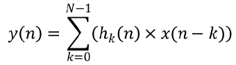
Where y — filter output; x — array of source data; hk — impulse responses; N — the number of impulse responses.
The instrument's price data serve as the source data, the number of impulse responses is set equal to the Nyquist interval. The impulse responses themselves are yet to be calculated. The ideal impulse responses for a low-pass filter can be calculated using the formula
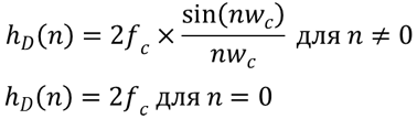
Where fc and wc are the cutoff frequency.
Unfortunately, our world is far from ideal. Therefore, a "real" impulse response is required. A weight function w (n) is needed to calculate it. There are several types of weight functions. Here, the Blackman function is used, which has the form
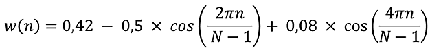
Where N is the number of filter elements.
To obtain the "real" impulse response, it is necessary to multiply the ideal impulse response with the corresponding weight function
![]()
Now that the calculation formulas are defined, let us create the CFLF class, where the impulse responses will be calculated and the input data will be filtered. To calculate the coefficients of the impulse response, let use create a public function CalcImpulses, which is passed the filtering period. Then the function algorithm repeats the above formulas. After that, it normalizes the impulse responses, bringing their sum to "1".
bool CFLF::CalcImpulses(int period)
  {
   if(period<20)
      return false;
   int N=(int)(period/2);
   if(ArraySize(cda_H)!=N)
      if(ArrayResize(cda_H,N)<N)
         return false;
   double H_id[],W[];
   if(ArrayResize(H_id,N)<N || ArrayResize(W,N)<N)
      return false;

   cd_Fs=1/(double)period;
   for (int i=0;i<N;i++)
     {
      if (i==0)
         H_id[i] = 2*M_PI*cd_Fs;
      else
         H_id[i] = MathSin(2*M_PI*cd_Fs*i )/(M_PI*i);

      W[i] = 0.42 - 0.5 * MathCos((2*M_PI*i) /( N-1)) + 0.08 * MathCos((4*M_PI*i) /( N-1));
      cda_H[i] = H_id[i] * W[i];
     }

   //Normalization
   double SUM=MathSum(cda_H);
   if(SUM==QNaN || SUM==0)
      return false;
   for (int i=0; i<N; i++)
      cda_H[i]/=SUM; //sum of coefficients equal to 1
   //---
   return true;
  }
2.3. Calculation of indicators FATL, SATL, RTFL, RSTL.
Once the impulse responses are obtained, we can proceed to calculation of the impulse indicator values. It will be convenient to obtain the values of the FATL, SATL, RFTL and RSTL indicators directly from the filter class.
Since different instances of the class will be used for the fast and slow filters, it is sufficient to create the AdaptiveTrendLine and ReferenceTrendLine functions in the class. The functions will be passed the used instrument, timeframe and shift relative to the current candle. The function will return the filtered value.
It should be noted that the ReferenceTrendLine function is essentially the same as the AdaptiveTrendLine function. The only difference is that ReferenceTrendLine is calculated with a shift value of the Nyquist period. Therefore, ReferenceTrendLine should calculate the Nyquist period and invoke AdaptiveTrendLine, specifying the appropriate shift relative to the current bar.
double CFLF::AdaptiveTrendLine(string symbol=NULL,ENUM_TIMEFRAMES timeframe=0,int shift=1)
  {
   string symb=(symbol==NULL ? _Symbol : symbol);
   int bars=ArraySize(cda_H);
   double values[];
   if(CopyClose(symb,timeframe,shift,bars,values)<=0)
      return QNaN;
   double mean=MathMean(values);
   double result=0;
   for(int i=0;i<bars;i++)
      result+=cda_H[i]*(values[bars-i-1]-mean);
   result+=mean;
   return result;
  }
//+------------------------------------------------------------------+
//|                                                                  |
//+------------------------------------------------------------------+
double CFLF::ReferenceTrendLine(string symbol=NULL,ENUM_TIMEFRAMES timeframe=0,int shift=1)
  {
   shift+=(int)(1/(2*cd_Fs));
   return AdaptiveTrendLine(symbol,timeframe,shift);
  }
The other indicators used are derivatives of the obtained values and will be calculated below.
3. Creating a trading signals module for the MQL5 Wizard
Today, I decided to digress from the usual way of writing experts and remind about the existence of the MQL Wizard in МetaТrader 5. This useful feature is a kind of constructor, which assembles an expert from premade modules. This allows you to easily create a new Expert Advisor, adding new features or removing unused ones. Therefore, I suggest embedding the considered Expert Advisor's decision-making algorithm into such a module. This method has already been discussed numerous times [4], [5]. Therefore, this article considers only the aspects related to the strategy.
Let us start by creating the CSignalATCF signal class based on the CExpertSignal, and include the previously created classes in it.
class CSignalATCF : public CExpertSignal { private: CSpectrum *Spectrum; //Class for spectrum calculation CFLF *FFLF; //Class of fast low frequency filter CFLF *SFLF; //Class of slow low frequency filterpublic: CSignalATCF(); ~CSignalATCF(); };
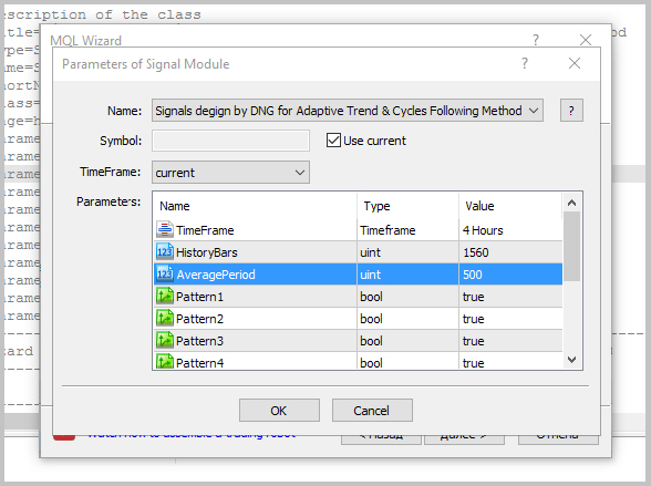
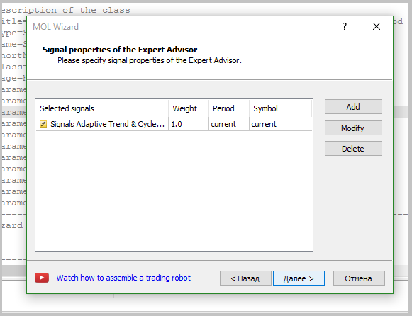
During the initialization, it is necessary to pass the module the instrument name, the used timeframe, the number of bars in history for the power spectral density analysis, as well as the number of bars for averaging (used in calculation of the RBCI and PCCI indicators). In addition, it is necessary to specify which of the patterns are to be used for opening positions. The general view of the module description will look as follows:
//--- wizard description start
//+---------------------------------------------------------------------------+
//| Description of the class                                                  |
//| Title=Signals design by DNG for Adaptive Trend & Cycles Following Method  |
//| Type=SignalAdvanced                                                       |
//| Name=Signals Adaptive Trend & Cycles Following Method                     |
//| ShortName=ATCF                                                            |
//| Class=CSignalATCF                                                         |
//| Page=https://www.mql5.com/ru/articles/3456                                |
//| Parameter=TimeFrame,ENUM_TIMEFRAMES,PERIOD_H4,Timeframe                   |
//| Parameter=HistoryBars,uint,1560,Bars in history to analysis               |
//| Parameter=AveragePeriod,uint,500,Period for RBCI and PCCI                 |
//| Parameter=Pattern1,bool,true,Use pattern 1                                |
//| Parameter=Pattern2,bool,true,Use pattern 2                                |
//| Parameter=Pattern3,bool,true,Use pattern 3                                |
//| Parameter=Pattern4,bool,true,Use pattern 4                                |
//| Parameter=Pattern5,bool,true,Use pattern 5                                |
//| Parameter=Pattern6,bool,true,Use pattern 6                                |
//| Parameter=Pattern7,bool,true,Use pattern 7                                |
//| Parameter=Pattern8,bool,true,Use pattern 8                                |
//+---------------------------------------------------------------------------+
//--- wizard description end
Now declare the required variables and functions:
class CSignalATCF : public CExpertSignal
  {
private:
   ENUM_TIMEFRAMES   ce_Timeframe;     //Timeframe
   uint              ci_HistoryBars;   //Bars in history to analysis
   uint              ci_AveragePeriod; //Period for RBCI and PCCI
   CSpectrum         *Spectrum;        //Class for spectrum calculation
   CFLF              *FFLF;            //Class of fast low frequency filter
   CFLF              *SFLF;            //Class of slow low frequency filter
   //--- Indicators data
   double             FATL, FATL1, FATL2;
   double             SATL, SATL1;
   double             RFTL, RFTL1, RFTL2;
   double             RSTL, RSTL1;
   double             FTLM, FTLM1, FTLM2;
   double             STLM, STLM1;
   double             RBCI, RBCI1, RBCI2;
   double             PCCI, PCCI1, PCCI2;
   //--- Patterns flags
   bool               cb_UsePattern1;
   bool               cb_UsePattern2;
   bool               cb_UsePattern3;
   bool               cb_UsePattern4;
   bool               cb_UsePattern5;
   bool               cb_UsePattern6;
   bool               cb_UsePattern7;
   bool               cb_UsePattern8;
   //---
   datetime           cdt_LastSpectrCalc;
   datetime           cdt_LastCalcIndicators;
   bool               cb_fast_calced;
   bool               cb_slow_calced;

   bool              CalculateIndicators(void);

public:
                     CSignalATCF();
                    ~CSignalATCF();
   //---
   void              TimeFrame(ENUM_TIMEFRAMES value);
   void              HistoryBars(uint value);
   void              AveragePeriod(uint value);
   void              Pattern1(bool value)                {  cb_UsePattern1=value;   }
   void              Pattern2(bool value)                {  cb_UsePattern2=value;   }
   void              Pattern3(bool value)                {  cb_UsePattern3=value;   }
   void              Pattern4(bool value)                {  cb_UsePattern4=value;   }
   void              Pattern5(bool value)                {  cb_UsePattern5=value;   }
   void              Pattern6(bool value)                {  cb_UsePattern6=value;   }
   void              Pattern7(bool value)                {  cb_UsePattern7=value;   }
   void              Pattern8(bool value)                {  cb_UsePattern8=value;   }
   //--- method of verification of settings
   virtual bool      ValidationSettings(void);
   //--- method of creating the indicator and timeseries
   virtual bool      InitIndicators(CIndicators *indicators);
   //--- methods of checking if the market models are formed
   virtual int       LongCondition(void);
   virtual int       ShortCondition(void);
  };
Create a function for calculating indicator values:
bool CSignalATCF::CalculateIndicators(void)
  {
   //--- Check time of last calculation
   datetime current=(datetime)SeriesInfoInteger(m_symbol.Name(),ce_Timeframe,SERIES_LASTBAR_DATE);
   if(current==cdt_LastCalcIndicators)
      return true;                  // Exit if data already calculated on this bar
   //--- Check for recalculation of spectrum
   MqlDateTime Current;
   TimeToStruct(current,Current);
   Current.hour=0;
   Current.min=0;
   Current.sec=0;
   datetime start_day=StructToTime(Current);

   if(!cb_fast_calced || !cb_slow_calced || (!PositionSelect(m_symbol.Name()) && start_day>cdt_LastSpectrCalc))
     {
      if(CheckPointer(Spectrum)==POINTER_INVALID)
        {
         Spectrum=new CSpectrum(ci_HistoryBars,m_symbol.Name(),ce_Timeframe);
         if(CheckPointer(Spectrum)==POINTER_INVALID)
           {
            cb_fast_calced=false;
            cb_slow_calced=false;
            return false;
           }
        }

      int fast,slow;
      if(Spectrum.GetPeriods(fast,slow))
        {
         cdt_LastSpectrCalc=(datetime)SeriesInfoInteger(m_symbol.Name(),ce_Timeframe,SERIES_LASTBAR_DATE);
         if(CheckPointer(FFLF)==POINTER_INVALID)
           {
            FFLF=new CFLF();
            if(CheckPointer(FFLF)==POINTER_INVALID)
               return false;
           }
         cb_fast_calced=FFLF.CalcImpulses(fast);
         if(CheckPointer(SFLF)==POINTER_INVALID)
           {
            SFLF=new CFLF();
            if(CheckPointer(SFLF)==POINTER_INVALID)
               return false;
           }
         cb_slow_calced=SFLF.CalcImpulses(slow);
        }
     }
   if(!cb_fast_calced || !cb_slow_calced)
      return false;                       // Exit on some error

   //--- Calculate indicators data
   int shift=StartIndex();
   double rbci[],pcci[],close[];
   if(ArrayResize(rbci,ci_AveragePeriod)<(int)ci_AveragePeriod || ArrayResize(pcci,ci_AveragePeriod)<(int)ci_AveragePeriod ||
      m_close.GetData(shift,ci_AveragePeriod,close)<(int)ci_AveragePeriod)
     {
      return false;
     }
   for(uint i=0;i<ci_AveragePeriod;i++)
     {
      double fatl=FFLF.AdaptiveTrendLine(m_symbol.Name(),ce_Timeframe,shift+i);
      double satl=SFLF.AdaptiveTrendLine(m_symbol.Name(),ce_Timeframe,shift+i);
      switch(i)
        {
         case 0:
            FATL=fatl;
            SATL=satl;
            break;
         case 1:
            FATL1=fatl;
            SATL1=satl;
            break;
         case 2:
            FATL2=fatl;
            break;
        }
      rbci[i]=fatl-satl;
      pcci[i]=close[i]-fatl;
     }
   RFTL=FFLF.ReferenceTrendLine(m_symbol.Name(),ce_Timeframe,shift);
   RSTL=SFLF.ReferenceTrendLine(m_symbol.Name(),ce_Timeframe,shift);
   RFTL1=FFLF.ReferenceTrendLine(m_symbol.Name(),ce_Timeframe,shift+1);
   RSTL1=SFLF.ReferenceTrendLine(m_symbol.Name(),ce_Timeframe,shift+1);
   RFTL2=FFLF.ReferenceTrendLine(m_symbol.Name(),ce_Timeframe,shift+2);
   FTLM=FATL-RFTL;
   STLM=SATL-RSTL;
   FTLM1=FATL1-RFTL1;
   STLM1=SATL1-RSTL1;
   FTLM2=FATL2-RFTL2;
   double dev=MathStandardDeviation(rbci);
   if(dev==0 || dev==QNaN)
      return false;
   RBCI=rbci[0]/dev;
   RBCI1=rbci[1]/dev;
   RBCI2=rbci[2]/dev;
   dev=MathAverageDeviation(pcci);
   if(dev==0 || dev==QNaN)
      return false;
   PCCI=pcci[0]/(dev*0.015);
   PCCI1=pcci[1]/(dev*0.015);
   PCCI2=pcci[2]/(dev*0.015);
   cdt_LastCalcIndicators=current;
  //---
   return true;
  }
Then code the patterns for opening and closing positions, specifying the corresponding weights (40 for closing and 80 for opening). Below is the function for opening long positions. The function for short positions is arranged similarly.
int CSignalATCF::LongCondition(void)
  {
   if(!CalculateIndicators() || m_open.GetData(1)>m_close.GetData(1))
      return 0;
   int result=0;
   //--- Close
   if(m_high.GetData(2)<m_close.GetData(1) || (STLM1<=0 && STLM>0) || (PCCI1<PCCI && PCCI1<=PCCI2) || (RBCI>RBCI1 && RBCI1>=RBCI2 && RBCI1<-1) || (RBCI1<=0 && RBCI>0))
      result=40;
   //--- Pattern 1
   if(cb_UsePattern1 && FTLM>0 && STLM>STLM1 && PCCI<100)
      result=80;
   else
   //--- Pattern 2
   if(cb_UsePattern2 && STLM>0 && FATL>FATL1 && FTLM>FTLM1 && RBCI>RBCI1 && (STLM>=STLM1 || (STLM<STLM1 && RBCI<1)))
      result=80;
   else
   //--- Pattern 3
   if(cb_UsePattern3 && STLM>0 && FATL>FATL1 && RBCI>RBCI1 && RBCI1<-1 && RBCI1<=RBCI2 && FTLM>FTLM1)
      result=80;
   else
   //--- Pattern 4
   if(cb_UsePattern4 && SATL>SATL1 && FATL>FATL1 && RBCI>RBCI1 && FTLM<FTLM1 && FTLM2<=FTLM1)
      result=80;
   else
   //--- Pattern 5
   if(cb_UsePattern5 && SATL>SATL1 && STLM>=0 && PCCI1<=-100 && PCCI1<PCCI && PCCI>-100 && RBCI>RBCI1 && RBCI1<=RBCI2 && RBCI1<-1)
      result=80;
   else
   //--- Pattern 6
   if(cb_UsePattern6 && SATL>SATL1 && STLM<0 && PCCI1<=-100 && PCCI>-100)
      result=80;
   else
   //--- Pattern 7
   if(cb_UsePattern7 && FATL>FATL1 && FATL1<=SATL1 && FATL>SATL && FATL1<=FATL2)
      result=80;
   //--- Pattern 8
   if(cb_UsePattern8 && FATL>FATL1 && FATL1<=SATL1 && FATL>SATL && FATL1<=RFTL1 && FATL>RFTL)
      result=80;

   return result;
  }
4. Creating the Expert Advisor with adaptive market following
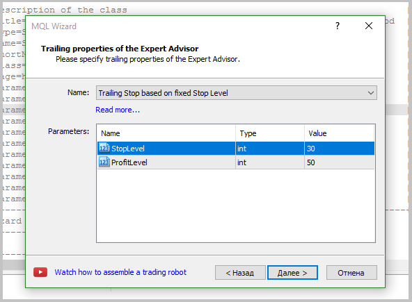
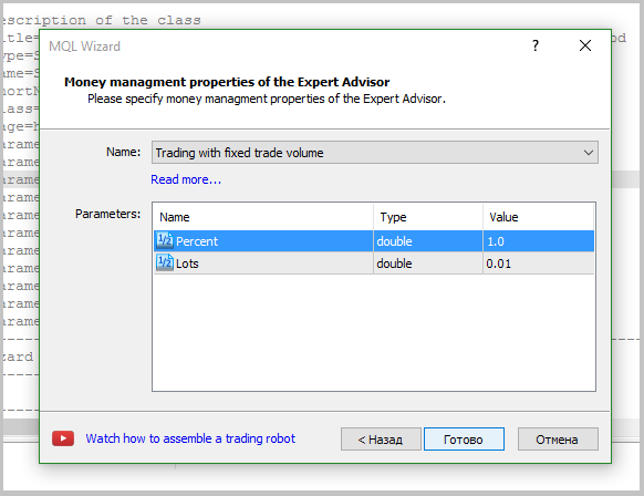
After creating the signal module, we can proceed to generation of the Expert Advisor. This article provides a detailed description of the process of creating an expert advisor using the Wizard. When creating the EA, only the trading signals module described above was used. In addition, trailing stop with a fixed number points was added. A fixed lot will be used when testing the strategy, which will allow evaluating the quality of the generated signals.
5. Testing the Expert Advisor.
Once the Expert Advisor is created, we can test the adaptive market following method in the Strategy Tester. When testing, it is mandatory to set the weight for opening the position at level 60 and the weight for closing the position at level 10.
5.1. Test without the use of stop loss, take profit and trailing stop.
To estimate the quality of the signals generated by the EA, the first test run was performed without the use of stop loss, take profit and trailing stop. Tests have been carried out on the H4 timeframe for 7 months of 2017.


Unfortunately, the first test showed that the application of the strategy without using stop loss is unprofitable.


The detailed analysis of the deals on the price chart showed two weak spots of the strategy:
- The Expert Advisor is unable to close the deals during rapid rebounds in time, which leads to loss of profit and unprofitable closure of the potentially profitable deals.
- The EA handles large movements well, but opens a number of unprofitable deals during flat movements.

5.2. Test with the use of stop loss and trailing stop.
To minimize the losses on the first point, stop loss and trailing stop were applied.


The results of the second test showed a reduction in the position holding time, a slight increase in the ratio of profitable trades, and a general tendency towards profit.


Nevertheless, the share of losing trades was 39.26%. And the second problem was still present (losing trades in a flat).
5.3. Test with the use of stop orders.
To reduce the losses associated with series of unprofitable trades in flat movements, a test with the use of stop orders was performed.


As a result of the third test run, the number of trades was almost halved, while the total profit increased, and the share of profitable trades increased to 44.57%.


Conclusion
The article considered the adaptive market following method. Testing has shown the potential of this strategy, but certain bottlenecks need to be eliminated for it to usable in the real market. Nevertheless, the method is viable. The source files and test results are provided in the attachment to the article.
References
- "Currency speculator", December 2000 - June 2001.
- Analysis of the Main Characteristics of Time Series.
- AR extrapolation of price - indicator for MetaTrader 5
- MQL5 Wizard: How to create a module of trading signals
- Create Your Own Trading Robot in 6 Steps!
- MQL5 Wizard: New Version
Programs used in the article:
| # | Name | Type | Description |
|---|---|---|---|
| 1 | Spectrum.mqh | Class library | Class for estimating the power spectral density of the analyzed instrument |
| 2 | FLF.mqh | Class library | Class for building a low-pass filter and filtering the initial data |
| 3 | SignalATCF.mqh | Class library | The module of trading signals based on the adaptive market following method |
| 4 | ATCF.mq5 | Expert Advisor | Expert Advisor based on the adaptive market following method |
| 5 | ACTF_Test.zip | Archive | The archive contains the results of testing the EA in the Strategy Tester. |