Using Discriminant Analysis to Develop Trading Systems
ArtemGaleev | 14 February, 2012
Introduction
One of the major tasks of technical analysis is to determine the direction in which the market will move in the near future. From a statistical standpoint, it boils down to selecting indicators and determining their values based on which it would be possible to divide the future market situation into two categories: 1) upward move, 2) downward move.
Discriminant analysis offers one of the ways to decide what kind of indicators and what values allow for better discrimination between these categories. In other words, discriminant analysis enables to build a model that will predict the market direction based on the data received from indicators.
Such analysis is however rather complicated requiring a great amount of data at the input. Therefore it is quite time-consuming to use it manually for analysis of the market situation. Fortunately, the emergence of the MQL5 language and statistical software has enabled us to automate data selection and preparation and application of the discriminant analysis.
This article gives an example of developing an EA for market data collection. It serves as a tutorial for application of the discriminant analysis for building prognostic model for the FOREX market in Statistica software.
1. What Is the Discriminant Analysis?
The discriminant analysis (hereinafter "DA") is one of the pattern recognition methods. Neural networks can be considered a special case of DA. DA is used in the majority of successful defense systems that are based on pattern recognition.
It allows to determine what variables divide (discriminate) the incoming data flow into groups and see the mechanism of such discrimination.
Let us have a look at a simplified example of using DA for the FOREX market. We have data values from Relative Strength Index (RSI), MACD and Relative Vigor Index (RVI) indicators and we need to predict the price direction. As a result of DA, we can get the following.
a. RVI indicator does not contribute to the forecast. So let us exclude it from the analysis.
b. DA has produced two discriminant equations:
- G1 = a1*RSI+b1*MACD+с1, the equation for cases where the price went up;
- G2 = a2*RSI+b2*MACD+с2, the equation for cases where the price went down.
Calculating G1 and G2 at the beginning of each bar, we predict that if G1 > G2, then the price will go up; whereas if G1 < G2, the price will go down.
DA may prove to be useful for initial acquaintance with neural networks. When using DA, we get equations similar to the ones calculated for operation of neural networks. This helps to better understand their structure and preliminarily determine whether it is worth using neural networks in your strategies.
2. Stages of the Discriminant Analysis
The analysis can be divided into several stages.
- Data preparation;
- Selection of the best variables from the prepared data;
- Analysis and testing of the resulting model using test data;
- Building of the model on the basis of discriminant equations.
Discriminant analysis is a part of almost all modern software packages designed for statistical data analysis. The most popular are Statistica (by StatSoft Inc.) and SPSS (by IBM Corporation). We will further consider the application of the discriminant analysis using Statistica software. The screenshots provided are obtained from Statistica version 8.0. These would look more or less the same in the earlier versions of the software. It should be noted that Statistica offers many other useful tools for the trader including neural networks.
2.1. Data Preparation
Data collection depends on a certain task at hand. Let us define the task as follows: using indicators, to predict the direction of the price chart on the bar following the bar with known values of indicators. An EA will be developed for data collection to save indicator values and price data into a file.
This shall be a CSV file with a following structure. Variables shall be arranged in columns where every column corresponds to a certain indicator. The rows shall contain consecutive measurements (cases), i.e. values of indicators for certain bars. In other words, the horizontal table headers contain indicators, the vertical table headers contain consecutive bars.
The table shall have a variable based on which the grouping will be made (the grouping variable). In our case, such variable will be based on the price change on the bar following the bar whose indicator values were obtained. The grouping variable shall contain the number of the group whose data is displayed in the same line. For example, number 1 for cases where the price went up and number 2 for cases where the price went down.
We will need values of the following indicators:
- Accelerator Oscillator;
- Bears Power;
- Bulls Power;
- Awesome Oscillator;
- Commodity Channel Index;
- DeMarker;
- Fractal Adaptive Moving Average;
- MACD;
- Relative Strength Index;
- Relative Vigor Index;
- Stochastic;
- Williams Percent Range.
The OnInit() function creates the indicators (obtains indicator handles) and MasterData.csv file where it saves the column data header:
//+------------------------------------------------------------------+
//| Expert initialization function                                   |
//+------------------------------------------------------------------+
int OnInit()
  {
//--- initialization of the indicators
   h_AC=iAC(Symbol(),Period());
   h_BearsPower=iBearsPower(Symbol(),Period(),BearsPower_PeriodBears);
   h_BullsPower=iBullsPower(Symbol(),Period(),BullsPower_PeriodBulls);
   h_AO=iAO(Symbol(),Period());
   h_CCI=iCCI(Symbol(),Period(),CCI_PeriodCCI,CCI_Applied);
   h_DeMarker=iDeMarker(Symbol(),Period(),DeM_PeriodDeM);
   h_FrAMA=iFrAMA(Symbol(),Period(),FraMA_PeriodMA,FraMA_Shift,FraMA_Applied);
   h_MACD=iMACD(Symbol(),Period(),MACD_PeriodFast,MACD_PeriodSlow,MACD_PeriodSignal,MACD_Applied);
   h_RSI=iRSI(Symbol(),Period(),RSI_PeriodRSI,RSI_Applied);
   h_RVI=iRVI(Symbol(),Period(),RVI_PeriodRVI);
   h_Stoch=iStochastic(Symbol(),Period(),Stoch_PeriodK,Stoch_PeriodD,Stoch_PeriodSlow,MODE_SMA,Stoch_Applied);
   h_WPR=iWPR(Symbol(),Period(),WPR_PeriodWPR);

   if(h_AC==INVALID_HANDLE || h_BearsPower==INVALID_HANDLE ||
      h_BullsPower==INVALID_HANDLE || h_AO==INVALID_HANDLE ||
      h_CCI==INVALID_HANDLE || h_DeMarker==INVALID_HANDLE ||
      h_FrAMA==INVALID_HANDLE || h_MACD==INVALID_HANDLE ||
      h_RSI==INVALID_HANDLE || h_RVI==INVALID_HANDLE ||
      h_Stoch==INVALID_HANDLE || h_WPR==INVALID_HANDLE)
     {
      Print("Error creating indicators");
      return(1);
     }

   ArraySetAsSeries(buf_AC,true);
   ArraySetAsSeries(buf_BearsPower,true);
   ArraySetAsSeries(buf_BullsPower,true);
   ArraySetAsSeries(buf_AO,true);
   ArraySetAsSeries(buf_CCI,true);
   ArraySetAsSeries(buf_DeMarker,true);
   ArraySetAsSeries(buf_FrAMA,true);
   ArraySetAsSeries(buf_MACD_m,true);
   ArraySetAsSeries(buf_MACD_s,true);
   ArraySetAsSeries(buf_RSI,true);
   ArraySetAsSeries(buf_RVI_m,true);
   ArraySetAsSeries(buf_RVI_s,true);
   ArraySetAsSeries(buf_Stoch_m,true);
   ArraySetAsSeries(buf_Stoch_s,true);
   ArraySetAsSeries(buf_WPR,true);


   FileHandle=FileOpen("MasterData2.csv",FILE_ANSI|FILE_WRITE|FILE_CSV|FILE_SHARE_READ,';');
   if(FileHandle!=INVALID_HANDLE)
     {
      Print("FileOpen OK");
      //--- saving names of the variables in the first line of the file for convenience of working with it
      FileWrite(FileHandle,"Time","Hour","Price","AC","dAC","Bears","dBears","Bulls","dBulls",
                "AO","dAO","CCI","dCCI","DeMarker","dDeMarker","FrAMA","dFrAMA","MACDm","dMACDm",
                "MACDs","dMACDs","MACDms","dMACDms","RSI","dRSI","RVIm","dRVIm","RVIs","dRVIs",
                "RVIms","dRVIms","Stoch_m","dStoch_m","Stoch_s","dStoch_s","Stoch_ms","dStoch_ms",
                "WPR","dWPR");
     }
   else
     {
      Print("FileOpen action failed. Error",GetLastError());
      ExpertRemove();
     }
//---
   return(0);
  }
The OnTick() event handler identifies new bars and saves data in the file.
The price behavior will be determined by the last completed bar and the values of the indicators will be obtained from the bar preceding the last completed bar. Apart from the absolute indicator value, we need to save the difference between the absolute and the preceding value in order to see the direction of the change. The names of such variables in the example provided will have prefix "d".
For signal line indicators, it is necessary to save the difference between the main and signal line as well as its dynamics. In addition, save the time of the new bar and the relevant hour value. This may come in handy for filtering the data by time.
Thus, we will take into account 37 indicators to build a forecasting model to estimate the price movement.
//+------------------------------------------------------------------+
//| Expert tick function                                             |
//| Monitoring the market situation and saving values                |
//| of the indicators into the file at the beginning of every new bar|
//+------------------------------------------------------------------+
void OnTick()
  {
//--- declaring a static variable of datetime type
   static datetime Prev_time;

//--- it will be used to store prices, volumes and spread of each bar
   MqlRates mrate[];
   MqlTick tickdata;

   ArraySetAsSeries(mrate,true);

//--- obtaining the recent quotes
   if(!SymbolInfoTick(_Symbol,tickdata))
     {
      Alert("Quote update error - error: ",GetLastError(),"!!");
      return;
     }
///--- copying data of the last 4 bars
   if(CopyRates(_Symbol,_Period,0,4,mrate)<0)
     {
      Alert("Historical quote copy error - error: ",GetLastError(),"!!");
      return;
     }
//--- if both time values are equal, there is no new bar
   if(Prev_time==mrate[0].time) return;
//--- saving the time in the static variable
   Prev_time=mrate[0].time;

//--- filling the arrays with values of the indicators
   bool copy_result=true;
   copy_result=copy_result && FillArrayFromBuffer1(buf_AC,h_AC,4);
   copy_result=copy_result && FillArrayFromBuffer1(buf_BearsPower,h_BearsPower,4);
   copy_result=copy_result && FillArrayFromBuffer1(buf_BullsPower,h_BullsPower,4);
   copy_result=copy_result && FillArrayFromBuffer1(buf_AO,h_AO,4);
   copy_result=copy_result && FillArrayFromBuffer1(buf_CCI,h_CCI,4);
   copy_result=copy_result && FillArrayFromBuffer1(buf_DeMarker,h_DeMarker,4);
   copy_result=copy_result && FillArrayFromBuffer1(buf_FrAMA,h_FrAMA,4);
   copy_result=copy_result && FillArraysFromBuffers2(buf_MACD_m,buf_MACD_s,h_MACD,4);
   copy_result=copy_result && FillArrayFromBuffer1(buf_RSI,h_RSI,4);
   copy_result=copy_result && FillArraysFromBuffers2(buf_RVI_m,buf_RVI_s,h_RVI,4);
   copy_result=copy_result && FillArraysFromBuffers2(buf_Stoch_m,buf_Stoch_s,h_Stoch,4);
   copy_result=copy_result && FillArrayFromBuffer1(buf_WPR,h_WPR,4);

//--- checking the accuracy of copying the data
   if(!copy_result==true)
     {
      Print("Data copy error");
      return;
     }

//--- saving to the file the price movement within the last two bars
//--- and the preceding values of the indicators
   if(FileHandle!=INVALID_HANDLE)
     {
      MqlDateTime tm;
      TimeCurrent(tm);
      uint Result=0;
      Result=FileWrite(FileHandle,TimeToString(TimeCurrent()),tm.hour, // time of the bar
                       (mrate[1].close-mrate[2].close)/_Point,       // difference between the closing prices of the last two bars
                       buf_AC[2],buf_AC[2]-buf_AC[3],                // value of the indicator on the preceding bar and its dynamics
                       buf_BearsPower[2],buf_BearsPower[2]-buf_BearsPower[3],
                       buf_BullsPower[2],buf_BullsPower[2]-buf_BullsPower[3],
                       buf_AO[2],buf_AO[2]-buf_AO[3],
                       buf_CCI[2],buf_CCI[2]-buf_CCI[3],
                       buf_DeMarker[2],buf_DeMarker[2]-buf_DeMarker[3],
                       buf_FrAMA[2],buf_FrAMA[2]-buf_FrAMA[3],
                       buf_MACD_m[2],buf_MACD_m[2]-buf_MACD_m[3],
                       buf_MACD_s[2],buf_MACD_s[2]-buf_MACD_s[3],
                       buf_MACD_m[2]-buf_MACD_s[2],buf_MACD_m[2]-buf_MACD_s[2]-buf_MACD_m[3]+buf_MACD_s[3],
                       buf_RSI[2],buf_RSI[2]-buf_RSI[3],
                       buf_RVI_m[2],buf_RVI_m[2]-buf_RVI_m[3],
                       buf_RVI_s[2],buf_RVI_s[2]-buf_RVI_s[3],
                       buf_RVI_m[2]-buf_RVI_s[2],buf_RVI_m[2]-buf_RVI_s[2]-buf_RVI_m[3]+buf_RVI_s[3],
                       buf_Stoch_m[2],buf_Stoch_m[2]-buf_Stoch_m[3],
                       buf_Stoch_s[2],buf_Stoch_s[2]-buf_Stoch_s[3],
                       buf_Stoch_m[2]-buf_Stoch_s[2],buf_Stoch_m[2]-buf_Stoch_s[2]-buf_Stoch_m[3]+buf_Stoch_s[3],
                       buf_WPR[2],buf_WPR[2]-buf_WPR[3]);

      if(Result==0)
        {
         Print("FileWrite action error ",GetLastError());
         ExpertRemove();
        }
     }

  }
After starting the EA, the MasterData.CSV file will be created in terminal_data_directory/MQL5/Files. When starting the EA in the tester, it will be located in terminal_data_directory/tester/Agent-127.0.0.1-3000/MQL5/Files. The file as obtained can already be used in Statistica.
An example of such file can be found in MasterData.CSV. The data was collected for EURUSD H1 from August 1, 2011 to October 1, 2011.
In order to open the file in Statistica, do as follows.
- In Statistica, go to menu File > Open, select the file type: Data files and open your file.
- Leave Delimited in the Text File Import Type window and click OK.
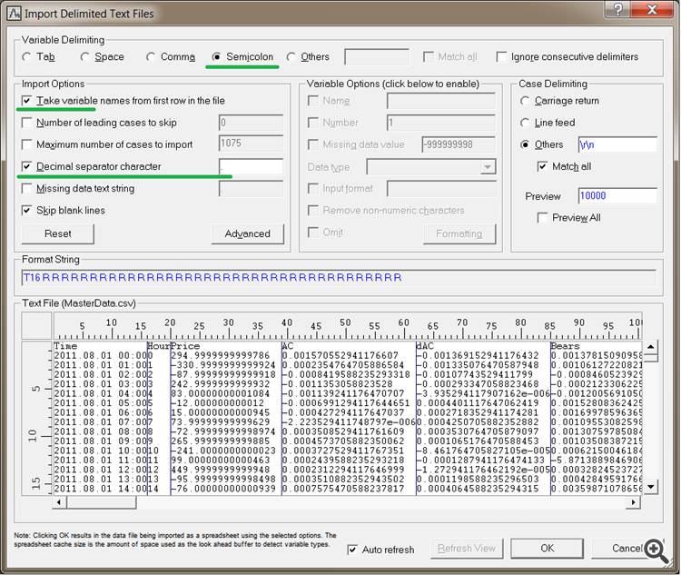
- Enable the underlined items in the opened window.
- Bear in mind to put the decimal point in the Decimal separator character field regardless of whether it is already there or not.
Fig. 1. Importing the file into Statistica
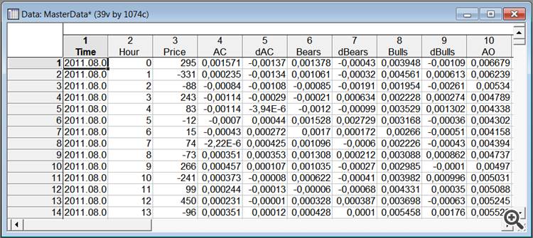
Click OK and the table containing our data is ready.
Fig. 2. Database in Statistica
Now create the grouping variable on the basis of the Price variable.
We will single out four groups depending on the price behavior:
- Over 200 points downwards;
- Less than 200 points downwards;
- Less than 200 points upwards;
- Over 200 points upwards.
In order to add a new variable, right-click on the AC column header and select the Add Variable option.
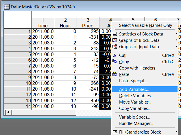
Fig. 3. Adding a new variable
Specify the name "Group" for the new variable in the opened window and add the formula for conversion of the Price variable to the number of groups.
The formula is as follows:
=iif(v3<=-200;1;0)+iif(v3<0 and v3>-200;2;0)+iif(v3>0 and v3<200;3;0)+iif(v3>=200;4;0)
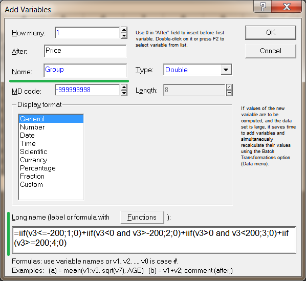
Fig. 4. Description of the variable
The file is ready for the discriminant analysis. An example of this file can be found in MasterData.STA.
2.2. Selection of the Best Variables
Run the discriminant analysis (Statistics->Multivariate Exploratory Techniques->Discriminant Analysis).
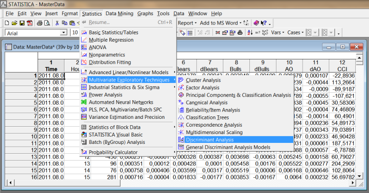
Fig. 5. Running the discriminant analysis
Click Variables in the opened window.
Select the grouping variable in the first field and all the variables based on which the grouping will be done - in the second field.
In our case, the Group variable is specified in the first field and all the variables obtained from the indicators as well as the additional variable Hour (the hour of receiving the data) - in the second field.
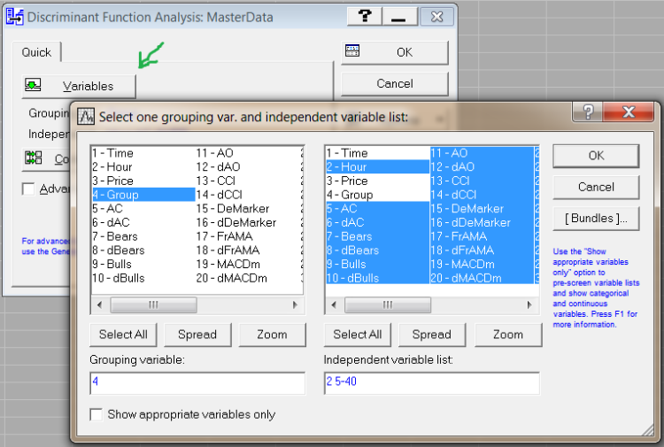
Fig. 6. Selection of variables
Click the Select Cases button (Figure 8). A window will open for selection of cases (data rows) which will be used in the discriminant analysis. Enable items as shown in the screenshot below (Figure 7).
Only the first 700 cases will be used for the analysis. The remaining ones will afterwards be used for testing of the resulting prognostic model. The numbers of cases are set via the variable V0. By specifying the cases in this manner, we set a sample of the training data for DA.
Then click OK.
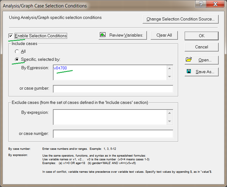
Fig. 7. Defining the training sample
Now let us select the groups for which our prognostic model will be built.
There is one issue that requires our attention. One of the weak points of DA is sensitivity to data outliers. Rare yet powerful events - in our case, price spikes- can distort the model. For example, following the unexpected news, the market responded with substantial movements lasting for a few hours. The values of technical indicators were in this case of little importance in the forecast yet they will be considered highly significant in DA as there was a marked price change. It is therefore advisable to check the data for outliers before running DA.
In order to exclude outliers from our example we will only analyze groups 2 and 3. Since there was a substantial price change in groups 1 and 4, there may be outliers in the indicator values.
So, click on Codes for grouping variable (Figure 8). And specify the numbers of groups for the analysis.
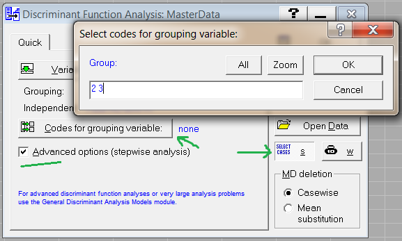
Fig. 8. Selection of groups for the analysis
Enable Advanced options. It will allow for the stepwise analysis that will be required at a later stage.
To run DA, click OK.
A message as below may pop up. This means that one of the selected variables is excessive and is substantially conditional on other variables, e.g. it is the sum of two other variables.
This is quite possible for the data flow obtained from the indicators. The presence of such variables affects the quality of the analysis. And they shall be removed. In order to do this, go back to the window for selection of variables for DA and identify the excessive variables by adding them one by one and running DA again and again.
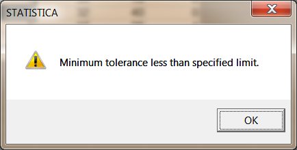
Fig. 9. Low tolerance value message
Then a window for selection of the DA method will open (Figure 10). Select Forward Stepwise in the drop-down list. Since the values of the indicators have little prognostic importance, the use of the stepwise analysis is preferred. And the model of group discrimination will automatically be built stepwise.
Specifically, at each step all variables will be reviewed and evaluated to determine which one will contribute most to the discrimination between the groups. That variable will then be included in the model and the process will start over again. All the variables that best discriminate between the data sample will be selected in the specified manner step by step.
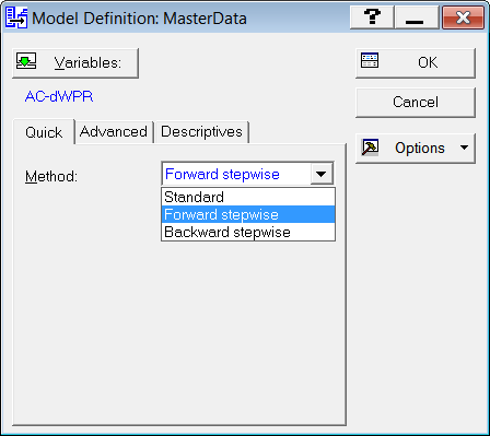
Fig. 10. Method selection
Click OK and a window will open informing you that DA was successfully completed.
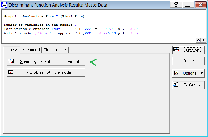
Fig. 11. Window of DA results
Click Summary: Variables in the model to see the list of variables included in the model following the stepwise analysis. These variables best discriminate between our groups. Note that the variables producing the accuracy of discrimination of over 95% (p<0.05) are displayed in red. The accuracy of discrimination with regard to other variables is lower. The model shall only include the variables producing the accuracy of discrimination of at least 95%.
However according to the "golden rule" of statistics, only the variables producing the accuracy of over 95% shall be used. We will therefore exclude from the analysis all variables that are not displayed in red. These are dBulls, Bulls, FrAMA, Hour. To exclude these variables, go back to the window where the stepwise analysis was selected and specify them in the window which will open after clicking Variables.
Repeat the analysis. By clicking the Summary: Variables in the model, we will again see that yet three other variables now appear as insignificant. These are DeMarker, Stoch_s, AO. We will also exclude them from the analysis.
As a result, we will have a model that includes the variables producing accurate discrimination between the groups (p<0.01).
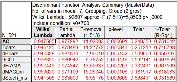
Fig. 12. Variables included in the model
Thus, only seven out of 37 variables were left in our example as being the most significant for the forecast.
This approach allows to select the key indicators on the basis of technical analysis for further development of custom trading systems, including the ones that utilize neural networks.
2.3. Analysis and Testing of the Resulting Model Using Test Data
Upon completion of DA, we obtained the prognostic model and the results of its application to training data.
To see the model and group discrimination results, open the Classification tab.
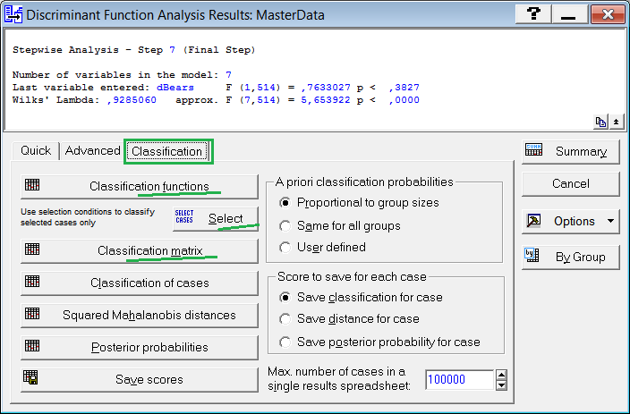
Fig. 13. Classification tab
Click Classification matrix to see the table containing the results of application of the model to training data.
The rows show the observed classifications. The columns contain the predicted classifications according to the model calculated. The cells that contain accurate predictions are marked in green and inaccurate predictions appear in red.
The first column displays the accuracy of prediction in %.
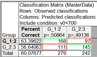
Fig. 14. Training data classification
The accuracy of prediction (Total) using training data turned out to be 60%.
Let us test the model using test data. To do this, click Select (Figure 13) and specify v0>700 following which the model will be checked within the range of data that was not used for building the model.
We will have the following:
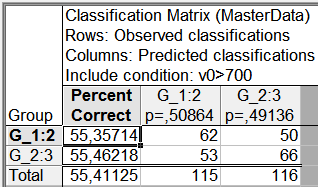
Fig. 15. Test data classification
The overall accuracy of prediction using the test sample turned out to be roughly at the same level reaching 55%. This is a fairly good level for the FOREX market.
2.4. Developing a Trading System
The prognostic model in DA is based on the system of linear equations according to which values of the indicators are classified into one group or the other.
In order to see the descriptions of these functions, go to the Classification tab in the window of DA results (Figure 13) and click Classification functions. You will see a window with a table containing the coefficients of discriminant equations.
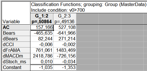
Fig. 16. Discriminant equations
Let us develop a system of two equations on the basis of the table data:
Group2 = 157.17*AC - 465.64*Bears + 82.24*dBears - 0.006*dCCI + 761.06*dFrAMA + 2418.79*dMACDm + 0.01*dStoch_ms - 1.035
Group3 = 527.11*AC - 641.97*Bears + 271.21*dBears - 0.002*dCCI + 1483.47*dFrAMA - 726.16*dMACDm - 0.034*dStoch_ms - 1.353
In order to use this model, insert the indicator values into the equations and calculate the Group value.
The forecast will concern the group whose Group value is higher. According to our example, if the Group2 value is bigger than that of Group3, it is predicted that within the next hour the price chart will most probably be moving downwards. The forecast will turn out to be quite the opposite in the case where the Group3 value is bigger than that of Group2.
It should be noted that the values of the indicators and period of analysis in our example were selected rather randomly. But even this amount of data was sufficient to demonstrate the potential and power of DA.
Conclusion
The discriminant analysis is a useful tool as applied to the FOREX market. It can be used to search and check the optimal set of variables allowing to classify the observed indicator values into different forecasts. It can also be utilized for building prognostic models.
The models built as a result of the discriminant analysis can easily be integrated into EAs which does not require a considerable developing experience. The discriminant analysis in itself is also relatively easy to use. The above step-by-step tutorial would suffice to analyze your own data.
More on the discriminant analysis can be found in the relevant section of the electronic textbook.
