Calculating the Hurst exponent
Dmitriy Piskarev | 3 April, 2017
Introduction
Defining the market dynamics is one of the main tasks of a trader. It is often too difficult to solve it using standard technical analysis tools. For example, МА or MACD may indicate a trend but we still need additional tools to evaluate its power and reliability. In the end, it may turn out to be a short-term spike that fades away quickly.
You probably know the axiom: In order to trade Forex successfully, we need to know a bit more than other market participants. In this case, you will be able to be one step ahead selecting the most favorable entry points and ensuring a trade profitability. Successful trading is a combination of several advantages, including placing buy/sell orders precisely during a trend reversal, skillful use of fundamental and technical data, as well as complete absence of emotions. All these are key elements of the successful trading career.
The fractal analysis may offer a comprehensive solution to many market evaluation issues. Fractals are often undeservedly neglected by traders and investors, although the fractal analysis of time series allows for efficient evaluation of a market trend and its reliability. The Hurst exponent is one of the basic values of fractal analysis.
Before moving on to calculation, let's briefly consider the main provisions of the fractal analysis and have a closer look at the Hurst exponent.
1. Fractal market hypothesis (FMH). Fractal analysis
Fractal is a mathematical set possessing the self-similarity property. A self-similar object is exactly or approximately similar to a part of itself (i.e. the whole has the same shape as one or more of the parts). The most vivid example of the fractal structure is a "fractal tree":

A self-similar object remains statistically similar in different scales — spatial or temporal.
When applied to markets, "fractal" means "recurrent" or "cyclical".
Fractal dimension defines how an object or a process fills the space and how its structure changes on various scales. When applying this definition to financial (or in our case — Forex) markets, we can state that the fractal dimension defines the degree of "irregularity" (variability) of a time series. Accordingly, a straight line has the dimension of d equal to one, random walk — d=1.5, while in case of a fractal time series 1<d<1.5 or 1.5<d<1.
"The purpose of the FMH is to give a model of investor behavior and market price movements that fits our observations... At any one time, prices may not reflect all available information, but only the information important to that investment horizon" — E. Peters, Fractal Market Analysis.
We are not going to dwell on the concept of fractality in details assuming that our readers already have an idea of this analytical method. The comprehensive description of its application to financial markets can be found in "The (Mis)behavior of Markets. A Fractal View of Financial Turbulence" by B. Mandelbrot and R. Hudson, as well as "Fractal Market Analysis" and "Chaos and Order in the Capital Markets: A New View of Cycles, Prices, and Market Volatility" by E. Peters.
2. R/S analysis and Hurst exponent
2.1. R/S analysis
The key parameter of the fractal analysis is the Hurst exponent used to study time series. The greater the delay between two similar value pairs in a time series, the lesser the Hurst exponent.
The exponent was introduced by Harold Edwin Hurst — an outstanding British hydrologist who worked on the Nile river dam project. In order to commence construction, Hurst needed to evaluate the fluctuations of the water level. Initially, it was assumed that the water inflow is a random, stochastic process. However, while studying records of the Nile floods for nine centuries, Hurst managed to detect patterns. This was the starting point in the study. It turned out that above average floods were followed by even stronger ones. After that, the process changed its direction and below average floods were followed by even weaker ones. These clearly were cycles with non-periodical duration.
The Hurst's statistical model is based on Albert Einstein's work about the Brownian motion providing the model of random walk of particles. The idea behind the theory is that a distance (R) walked by a particle increases proportionally to the square root of the time (T):
![]()
Let's re-phrase the equation: in case of a large number of tests, variation range (R) is equal to the square root of the number of tests (T). This equation was used by Hurst when proving that the Nile floods are not random.
In order to form his method, the hydrologist used the X1..Xn time series of the river floods. The following algorithm called the rescaled range method or R/S analysis later was then applied:
- Calculating the average value, Xm, of the X1..Xn series
- Calculating the standard series deviation, S
- Normalization of the series by deducting the average value, Zr (where r=1..n), from each value
- Creating a cumulative time series Y1=Z1+Zr, where r=2..n
- Calculating the magnitude of the cumulative time series R=max(Y1..Yn)-min(Y1..Yn)
- Dividing the magnitude of the cumulative time series by the standard deviation (S).
Hurst expanded the Einstein's equation converting it to the more general form:
![]()
where с is a constant.
Generally, the R/S value changes the scale with increasing of the time increment according to the dependence degree equal to H which is the Hurst exponent.
According to Hurst, H would have been equal to 0.5 if the flood process had been random. However, during his observations, he found out that H=0.91! This means that the normalized magnitude changes faster than the square root of time. In other words, the system passes a longer distance than a random process meaning that past events have a significant impact on present and future ones.
2.2. Applying the theory to markets
Subsequently, the Hurst exponent calculation method was applied to financial and stock markets. It includes normalizing data to the zero average and single standard deviation to compensate for the inflation component. In other words, we are dealing with the R/S analysis again.
How to interpret the Hurst exponent on the markets?1. If the Hurst exponent is between 0.5 and 1, and it differs from the expected value by two and more standard deviations, the process is characterized by a long-term memory. In other words, there is persistence.
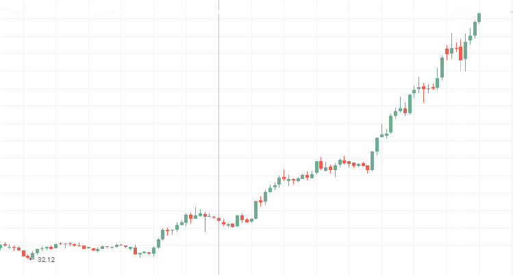
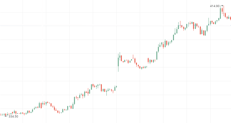
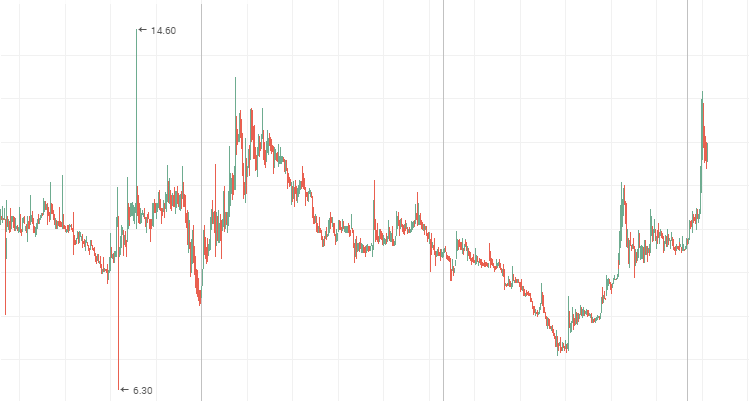
This means all the following results strongly depend on the previous ones within a certain time period. The quote charts of the most reliable and influential companies represent the most illustrative persistent time series. US corporations like Apple, GE, Boeing, as well as Russian ones like Rosneft, Aeroflot and VTB can be named among others. The quote charts of these companies are displayed below. I believe, every investor can discern a familiar picture while looking at this charts — every new High and Low is higher than the previous one.
Aeroflot stock prices:
Rosneft stock prices:
VTM stock prices, downward persistent time series
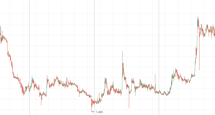
2. If the Hurst exponent is different from the expected value by two or more standard deviations in absolute value and is between 0 and 0.5, this means we are dealing with anti-persistent time series.
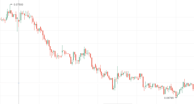
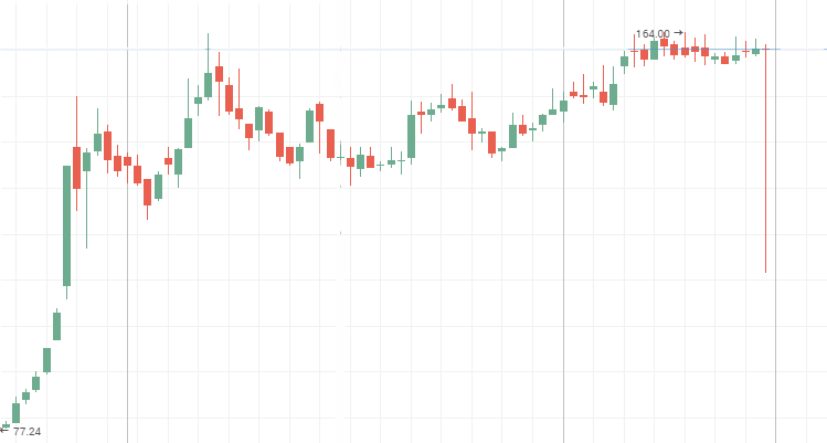
The system changes faster than a random one, i.e. it is prone to small but frequent changes. The anti-persistent process can be clearly seen on the 2-tier stock charts. During flat movements, "blue chip" price charts demonstrate anti-persistent behavior as well. Stock charts of Mechel, AvtoVAZ and Lenenergo provided below are vivid examples of anti-persistent time series.
Mechel preferred stocks:
AvtoVAZ common stocks during a flat
Lenenergo:
3. If the Hurst exponent is 0.5 or its value is different from the expected value by less than two standard deviations, the process is considered to be a random walk. No short- or long-term cyclical dependencies are expected. In trading, this means that technical analysis is of no much help since the current values are almost unaffected by the previous ones. So, it is better to use the fundamental analysis.
The sample Hurst exponents for stock market instruments (securities of various corporations, industrial companies and goods) are provided in the table below. The calculation has been performed for the last 7 years. The "blue chips" have low exponent values demonstrating consolidation phase during the financial crisis. Interestingly, many 2-tier securities show persistence demonstrating robustness against the crisis.
| Name | Hurst exponent, H |
|---|---|
| Gazprom |
0.552 |
| VTB |
0.577 |
| Magnit |
0.554 |
| MTS |
0.543 |
| Rosneft |
0.648 |
| Aeroflot | 0.624 |
| Apple | 0.525 |
| GE | 0.533 |
| Boeing | 0.548 |
| Rosseti |
0.650 |
| Raspadskaya |
0.656 |
| TGC-1 |
0.641 |
| Tattelecom |
0.582 |
| Lenenergo |
0.642 |
| Mechel |
0.635 |
| AvtoVAZ |
0.574 |
| Petrol | 0.586 |
| Tin | 0.565 |
| Palladium | 0.564 |
| Natural gas | 0.560 |
| Nickel | 0.580 |
3. Defining cycles. Memory in the fractal analysis
How can we be sure that our results are not random (trivial)? In order to answer this question, we should first study the RS analysis assuming that the analyzed system is of random nature. In other words, we should check the validity of the null hypothesis stating that the process is a random walk, and its structure is independent and normally distributed.
3.1. Calculating the expected R/S analysis value
Let's introduce the concept of an expected R/S analysis value.
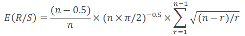
In 1976, Anis and Lloyd derived an equation expressing a necessary expected value:
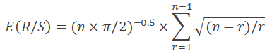
where n is a number of observations, while r represents integers from 1 to n-1.
As stated in "Fractal Market Analysis", provided equation is valid only for n>20. For n<20, use the following equation:
All is pretty simple:
- calculate an expected value for each number of observations and display an obtained Log(E(R/S)) graph from Log(N) together with Log(R/S) from Log(N);
- calculated an expected dispersion of the Hurst exponent using the equation that is well known in the statistical theory
![]()
where H is a Hurst exponent;
N – number of observations in the sample;
3. check the relevance of the obtained Hurst ratio by evaluating the number of standard deviations, by which H exceeds E(H). The result is considered relevant if the relevance exceeds 2 in absolute magnitude.
3.2. Defining cycles
Let's consider the following example. Plot two graphs for RS statistics and expected value E(R/S) and compare them with the market dynamics to find out whether calculation results match the quotes movement.
In his works, Peters notes that the best way to define the presence of a cycle is to build a V-statistics graph in a logarithmic scale based on a logarithm of a number of observations in a subgroup.
The obtained results are easy to evaluate:
- if a chart on a logarithmic scale is a horizontal line on both axes, then we are dealing with an independent random process;
- if the graph has a positive upward slope angle, we are dealing with a persistent process. As I have already mentioned, this means that R/S scale changes occur faster than the square root of time;
- and finally, if the graph shows a downward trend, we are dealing with an anti-persistent process.
3.3. The concept of memory in the fractal analysis and how to define its depth
For further understanding of the fractal analysis, let's introduce the concept of memory.
I have already mentioned long-term and short-term memory. In fractal analysis, the memory is a time interval, during which the market remembers the past and considers its impact on the present and future events. This time interval is a memory depth, which to some extent contains the entire power and specifics of the fractal analysis. This data is vital for technical analysis when defining the relevance of a past technical pattern.
No excessive processing power is required to determine a memory depth. Only a simple visual analysis of the V statistics logarithm graph is sufficient.
- Draw a trend line along all the graph points involved.
- Make sure that the curve is not horizontal.
- Define the curve peaks or the points where the function reached its maximum values. These maximum values serve as the first warning of an existing cycle.
- Define the X coordinate of the graph on a logarithmic scale and convert the number to make it easy to comprehend: Period length = exp^ (Period length on a logarithmic scale). Thus, if you analyzed 12000 GBPUSD hour data and obtained 8.2 on a logarithmic scale, the cycle is equal to exp^8.2=3772 hours or 157 days.
- Any true cycles should be saved on the same time interval but with another timeframe as a base. For example, in p. 4, we investigated 12000 GBPUSD hour data and suggested that a cycle of 157 days is present. Switch to H4 and analyze 12000/4=3000 data. If the 157-day cycle actually exists, then your assumptions are most probably correct. If not, then you might be able to find shorter memory cycles.
3.4. Actual Hurst exponent values for currency pairs
We have finished the introduction of the fractal analysis theory basic principles. Before proceeding to the immediate implementation of the RS analysis using MQL5 programming language, let's consider some more examples.
The table below shows Hurst exponent values for 11 Forex currency pairs on various timeframes and number of bars. Ratios are calculated by solving the regression using the least square (LS) method. As we can see, most currency pairs support the persistent process, although there are anti-persistent ones as well. But is this result significant? Can we trust these numbers? We will discuss this later.
Table 1. Analyzing the Hurst exponent for 2000 bars
| Symbol | H (D1) | H (H4) | H (H1) | H(15M) | H (5M) | E(H) |
|---|---|---|---|---|---|---|
| EURUSD | 0.545 | 0,497 | 0.559 | 0.513 | 0.567 | 0.577 |
| EURCHF | 0.520 | 0.468 | 0.457 | 0.463 | 0.522 | 0.577 |
| EURJPY | 0.574 | 0.501 | 0.527 | 0.511 | 0.546 | 0.577 |
| EURGBP | 0.553 | 0.571 | 0.540 | 0.562 | 0.550 | 0.577 |
| EURRUB | insufficient bars | 0.536 | 0.521 | 0.543 | 0.476 | 0.577 |
| USDJPY | 0.591 | 0.563 | 0.583 | 0.519 | 0.565 | 0.577 |
| USDCHF | insufficient bars | 0.509 | 0.564 | 0.517 | 0.545 | 0.577 |
| USDCAD | 0.549 | 0.569 | 0.540 | 0.519 | 0.565 | 0.577 |
| USDRUB | 0.582 | 0.509 | 0.564 | 0.527 | 0.540 | 0.577 |
| AUDCHF | 0.522 | 0.478c | 0.504 | 0.506 | 0.509 | 0.577 |
| GBPCHF | 0.554 | 0.559 | 0.542 | 0.565 | 0.559 | 0.577 |
Table 2. Analyzing the Hurst exponent for 400 bars
| Symbol | H (D1) | H (H4) | H (H1) | H(15M) | H (5M) | E(H) |
|---|---|---|---|---|---|---|
| EURUSD | 0.545 | 0,497 | 0.513 | 0.604 | 0.617 | 0.578 |
| EURCHF | 0.471 | 0.460 | 0.522 | 0.603 | 0.533 | 0.578 |
| EURJPY | 0.545 | 0.494 | 0.562 | 0.556 | 0.570 | 0.578 |
| EURGBP | 0.620 | 0.589 | 0.601 | 0.597 | 0.635 | 0.578 |
| EURRUB | 0.580 | 0.551 | 0.478 | 0.526 | 0.542 | 0.578 |
| USDJPY | 0.601 | 0.610 | 0.568 | 0.583 | 0.593 | 0.578 |
| USDCHF | 0.505 | 0.555 | 0.501 | 0.585 | 0.650 | 0.578 |
| USDCAD | 0.590 | 0.537 | 0.590 | 0.587 | 0.631 | 0.578 |
| USDRUB | 0.563 | 0.483 | 0.465 | 0.531 | 0.502 | 0.578 |
| AUDCHF | 0.443 | 0.472 | 0.505 | 0.530 | 0.539 | 0.578 |
| GBPCHF | 0.568 | 0.582 | 0.616 | 0.615 | 0.636 | 0.578 |
Table 3. Hurst exponent calculation results for M15 and M5
| Symbol | H (15M) | Significance | H (5M) | Significance | E(H) |
|---|---|---|---|---|---|
| EURUSD | 0.543 | insignificant | 0.542 | insignificant | 0.544 |
| EURCHF | 0.484 | significant | 0.480 | significant | 0.544 |
| EURJPY | 0.513 | insignificant | 0.513 | insignificant | 0.544 |
| EURGBP | 0.542 | insignificant | 0.528 | insignificant | 0.544 |
| EURRUB | 0.469 | significant | 0.495 | significant | 0.544 |
| USDJPY | 0.550 | insignificant | 0.525 | insignificant | 0.544 |
| USDCHF | 0.551 | insignificant | 0.525 | insignificant | 0.544 |
| USDCAD | 0.519 | insignificant | 0.550 | insignificant | 0.544 |
| USDRUB | 0.436 | significant | 0.485 | significant | 0.544 |
| AUDCHF | 0.518 | insignificant | 0.499 | significant | 0.544 |
| GBPCHF | 0.533 | insignificant | 0.520 | insignificant | 0.544 |
E. Peters recommends analyzing some basic timeframe and use it to search for a time series possessing cyclic dependencies. Then, the analyzed time interval is divided into a lesser number of bars by changing a timeframe and "fitting" a history depth. This implies the following:
If the cycle is present on the base timeframe, its validity can probably be proven if the same cycle is found in a different division.
Using different combinations of available bars, we can find non-periodic cycles. Their length can eliminate any doubts concerning the usefulness of past technical indicator signals.
4. From theory to practice
Now that we have obtained basic knowledge about the fractal analysis, the Hurst exponent and interpretation of its values, it is time to implement the idea using MQL5.
Let's define the technical requirements the following way: we need a program that calculates the Hurst exponent for 1000 history bars on a specified pair.
Step 1. Create a new script

We receive a "stub" to be filled with data. Also, add the #property script_show_inputs since we will have to select a currency pair at the entry.
//| New.mq5 |
//| Copyright 2016, Piskarev D.M. |
//| piskarev.dmitry25@gmail.com |
//+------------------------------------------------------------------+
#property copyright "Copyright 2016, Piskarev D.M."
#property link "piskarev.dmitry25@gmail.com"
#property version "1.00"
#property script_show_inputs
//+------------------------------------------------------------------+
//| Script program start function |
//+------------------------------------------------------------------+
void OnStart()
{
//---
}
//+------------------------------------------------------------------+
Step 2. Set the close price array and check if 1001 history bars are currently available for the selected currency pair.
Why do we use 1001 bars when 1000 bars are set in the technical requirements? Answer: The data on the previous value is required to form the array of logarithmic returns.
int copied=CopyClose(symbol,timeframe,0,barscount1+1,close); //copy Close prices of the selected pair to
//close[] array
ArrayResize(close,1001); //set the array size
ArraySetAsSeries(close,true);
if(bars<1001) //create a condition for the presence of 1001 history bars
{
Comment("Too few bars are available! Try another timeframe.");
Sleep(10000); //delay the label for 10 seconds
Comment("");
return;
}
Step 3. Create the array of logarithmic returns.
It is assumed that the LogReturns array has already been declared and the ArrayResize(LogReturns,1001) string is present
LogReturns[i]=MathLog(close[i-1]/close[i]);
Step 4. Calculate the Hurst exponent.
For correct analysis, we need to divide the analyzed amount of history bars by subgroups so that the number of elements in each of them is not less than 10. In other words, we need to find dividers for 1000 with their values exceeding ten. There are 11 such dividers:
num1=10;
num2=20;
num3=25;
num4=40;
num5=50;
num6=100;
num7=125;
num8=200;
num9=250;
num10=500;
num11=1000;
Since we calculate data for RS statistics 11 times, it would be reasonable to develop a custom function for that. The final and initial indices of the subgroup, for which the RS statistics is calculated, as well as the number of analyzed bars are used as the function parameters. The algorithm is completely similar to the one described in the beginning of the article.
//| R/S calculation function |
//+----------------------------------------------------------------------+
double RSculc(int bottom,int top,int barscount)
{
Sum=0.0; //Initial sum is zero
DevSum=0.0; //Initial sum of the accumulated
//deviations is zero
//--- Calculate the sum of returns
for(int i=bottom; i<=top; i++)
Sum=Sum+LogReturns[i]; //Accumulate the sum
//--- Calculate the average
M=Sum/barscount;
//--- Calculate accumulated deviations
for(int i=bottom; i<=top; i++)
{
DevAccum[i]=LogReturns[i]-M+DevAccum[i-1];
StdDevMas[i]=MathPow((LogReturns[i]-M),2);
DevSum=DevSum+StdDevMas[i]; //Component for calculating a deviation
if(DevAccum[i]>MaxValue) //If the array value is less than a
MaxValue=DevAccum[i]; //maximum one, the DevAccum array element value is assigned to
//the maximum value
if(DevAccum[i]<MinValue) //Logic is identical
MinValue=DevAccum[i];
}
//--- Calculate R amplitude and S deviation
R=MaxValue-MinValue; //Amplitude is a difference between the maximum and
MaxValue=0.0; MinValue=1000; //minimum values
S1=MathSqrt(DevSum/barscount); //Calculate the standard deviation
//--- Calculate the R/S parameter
if(S1!=0)RS=R/S1; //Eliminate zero divide error
// else Alert("Zero divide!");
return(RS); //Return RS statistics value
}
Calculate using switch-case.
for(int A=1; A<=11; A++) //cycle allows us to shorten the code
{ //besides, we consider all possible dividers
switch(A)
{
case 1: // 100 groups containing 10 elements each
{
ArrayResize(rs1,101);
RSsum=0.0;
for(int j=1; j<=100; j++)
{
rs1[j]=RSculc(10*j-9,10*j,10); //call the RScuclc custom function
RSsum=RSsum+rs1[j];
}
RS1=RSsum/100;
LogRS1=MathLog(RS1);
}
break;
case 2: // 50 groups containing 20 elements each
{
ArrayResize(rs2,51);
RSsum=0.0;
for(int j=1; j<=50; j++)
{
rs2[j]=RSculc(20*j-19,20*j,20); //call the RScuclc custom function
RSsum=RSsum+rs2[j];
}
RS2=RSsum/50;
LogRS2=MathLog(RS2);
}
break;
...
...
...
case 9: // 125 and 16 groups
{
ArrayResize(rs9,5);
RSsum=0.0;
for(int j=1; j<=4; j++)
{
rs9[j]=RSculc(250*j-249,250*j,250);
RSsum=RSsum+rs9[j];
}
RS9=RSsum/4;
LogRS9=MathLog(RS9);
}
break;
case 10: // 125 and 16 groups
{
ArrayResize(rs10,3);
RSsum=0.0;
for(int j=1; j<=2; j++)
{
rs10[j]=RSculc(500*j-499,500*j,500);
RSsum=RSsum+rs10[j];
}
RS10=RSsum/2;
LogRS10=MathLog(RS10);
}
break;
case 11: //200 and 10 groups
{
RS11=RSculc(1,1000,1000);
LogRS11=MathLog(RS11);
}
break;
}
}
Step 5. Custom function for calculating the linear regression using the least square (LS) method.
The input parameters are the values of the calculated RS statistics components.
double RegCulc1000(double Y1,double Y2,double Y3,double Y4,double Y5,double Y6,
double Y7,double Y8,double Y9,double Y10,double Y11)
{
double SumY=0.0;
double SumX=0.0;
double SumYX=0.0;
double SumXX=0.0;
double b=0.0;
double N[]; //array to store the divider logarithms
double n={10,20,25,40,50,100,125,200,250,500,1000} //divider array
//---Calculate N ratios
for (int i=0; i<=10; i++)
{
N[i]=MathLog(n[i]);
SumX=SumX+N[i];
SumXX=SumXX+N[i]*N[i];
}
SumY=Y1+Y2+Y3+Y4+Y5+Y6+Y7+Y8+Y9+Y10+Y11;
SumYX=Y1*N1+Y2*N2+Y3*N3+Y4*N4+Y5*N5+Y6*N6+Y7*N7+Y8*N8+Y9*N9+Y10*N10+Y11*N11;
//---Calculate the Beta regression ratio or the necessary Hurst exponent
b=(11*SumYX-SumY*SumX)/(11*SumXX-SumX*SumX);
return(b);
}
Step 6. Custom function for calculating expected RS statistics values. Calculation logic is explained in the theoretical part.
//| Function for calculating expected E(R/S) values |
//+----------------------------------------------------------------------+
double ERSculc(double m) //m - 1000 dividers
{
double e;
double nSum=0.0;
double part=0.0;
for(int i=1; i<=m-1; i++)
{
part=MathPow(((m-i)/i), 0.5);
nSum=nSum+part;
}
e=MathPow((m*pi/2),-0.5)*nSum;
return(e);
}
The complete program code may look as follows:
//| hurst_exponent.mq5 |
//| Copyright 2016, Piskarev D.M. |
//| piskarev.dmitry25@gmail.com |
//+------------------------------------------------------------------+
#property copyright "Copyright 2016, Piskarev D.M."
#property link "piskarev.dmitry25@gmail.com"
#property version "1.00"
#property script_show_inputs
#property strict
input string symbol="EURUSD"; // Symbol
input ENUM_TIMEFRAMES timeframe=PERIOD_D1; // Timeframe
double LogReturns[],N[],
R,S1,DevAccum[],StdDevMas[];
int num1,num2,num3,num4,num5,num6,num7,num8,num9,num10,num11;
double pi=3.14159265358979323846264338;
double MaxValue=0.0,MinValue=1000.0;
double DevSum,Sum,M,RS,RSsum,Dconv;
double RS1,RS2,RS3,RS4,RS5,RS6,RS7,RS8,RS9,RS10,RS11,
LogRS1,LogRS2,LogRS3,LogRS4,LogRS5,LogRS6,LogRS7,LogRS8,LogRS9,
LogRS10,LogRS11;
double rs1[],rs2[],rs3[],rs4[],rs5[],rs6[],rs7[],rs8[],rs9[],rs10[],rs11[];
double E1,E2,E3,E4,E5,E6,E7,E8,E9,E10,E11;
double H,betaE;
int bars=Bars(symbol,timeframe);
double D,StandDev;
//+------------------------------------------------------------------+
//| Script program start function |
//+------------------------------------------------------------------+
void OnStart()
{
double close[]; //Declare the dynamic Close price array
int copied=CopyClose(symbol,timeframe,0,1001,close); //Copy a Close price of the selected pair to
//close[] array
ArrayResize(close,1001); //Set the array size
ArraySetAsSeries(close,true);
if(bars<1001) //Create a condition for the presence of 1001 history bars
{
Comment("Too few bars are available! Try another timeframe.");
Sleep(10000); //Delay the label for 10 seconds
Comment("");
return;
}
//+------------------------------------------------------------------+
//| Preparing the arrays |
//+------------------------------------------------------------------+
ArrayResize(LogReturns,1001);
ArrayResize(DevAccum,1001);
ArrayResize(StdDevMas,1001);
//+------------------------------------------------------------------+
//| Array of logarithmic returns |
//+------------------------------------------------------------------+
for(int i=1;i<=1000;i++)
LogReturns[i]=MathLog(close[i-1]/close[i]);
//+------------------------------------------------------------------+
//| |
//| R/S analysis |
//| |
//+------------------------------------------------------------------+
//--- Set the number of elements in each subgroup
num1=10;
num2=20;
num3=25;
num4=40;
num5=50;
num6=100;
num7=125;
num8=200;
num9=250;
num10=500;
num11=1000;
//--- Calculate the composite Log(R/S)
for(int A=1; A<=11; A++)
{
switch(A)
{
case 1:
{
ArrayResize(rs1,101);
RSsum=0.0;
for(int j=1; j<=100; j++)
{
rs1[j]=RSculc(10*j-9,10*j,10);
RSsum=RSsum+rs1[j];
}
RS1=RSsum/100;
LogRS1=MathLog(RS1);
}
break;
case 2:
{
ArrayResize(rs2,51);
RSsum=0.0;
for(int j=1; j<=50; j++)
{
rs2[j]=RSculc(20*j-19,20*j,20);
RSsum=RSsum+rs2[j];
}
RS2=RSsum/50;
LogRS2=MathLog(RS2);
}
break;
case 3:
{
ArrayResize(rs3,41);
RSsum=0.0;
for(int j=1; j<=40; j++)
{
rs3[j]=RSculc(25*j-24,25*j,25);
RSsum=RSsum+rs3[j];
}
RS3=RSsum/40;
LogRS3=MathLog(RS3);
}
break;
case 4:
{
ArrayResize(rs4,26);
RSsum=0.0;
for(int j=1; j<=25; j++)
{
rs4[j]=RSculc(40*j-39,40*j,40);
RSsum=RSsum+rs4[j];
}
RS4=RSsum/25;
LogRS4=MathLog(RS4);
}
break;
case 5:
{
ArrayResize(rs5,21);
RSsum=0.0;
for(int j=1; j<=20; j++)
{
rs5[j]=RSculc(50*j-49,50*j,50);
RSsum=RSsum+rs5[j];
}
RS5=RSsum/20;
LogRS5=MathLog(RS5);
}
break;
case 6:
{
ArrayResize(rs6,11);
RSsum=0.0;
for(int j=1; j<=10; j++)
{
rs6[j]=RSculc(100*j-99,100*j,100);
RSsum=RSsum+rs6[j];
}
RS6=RSsum/10;
LogRS6=MathLog(RS6);
}
break;
case 7:
{
ArrayResize(rs7,9);
RSsum=0.0;
for(int j=1; j<=8; j++)
{
rs7[j]=RSculc(125*j-124,125*j,125);
RSsum=RSsum+rs7[j];
}
RS7=RSsum/8;
LogRS7=MathLog(RS7);
}
break;
case 8:
{
ArrayResize(rs8,6);
RSsum=0.0;
for(int j=1; j<=5; j++)
{
rs8[j]=RSculc(200*j-199,200*j,200);
RSsum=RSsum+rs8[j];
}
RS8=RSsum/5;
LogRS8=MathLog(RS8);
}
break;
case 9:
{
ArrayResize(rs9,5);
RSsum=0.0;
for(int j=1; j<=4; j++)
{
rs9[j]=RSculc(250*j-249,250*j,250);
RSsum=RSsum+rs9[j];
}
RS9=RSsum/4;
LogRS9=MathLog(RS9);
}
break;
case 10:
{
ArrayResize(rs10,3);
RSsum=0.0;
for(int j=1; j<=2; j++)
{
rs10[j]=RSculc(500*j-499,500*j,500);
RSsum=RSsum+rs10[j];
}
RS10=RSsum/2;
LogRS10=MathLog(RS10);
}
break;
case 11:
{
RS11=RSculc(1,1000,1000);
LogRS11=MathLog(RS11);
}
break;
}
}
//+----------------------------------------------------------------------+
//| Calculate the Hurst exponent |
//+----------------------------------------------------------------------+
H=RegCulc1000(LogRS1,LogRS2,LogRS3,LogRS4,LogRS5,LogRS6,LogRS7,LogRS8,
LogRS9,LogRS10,LogRS11);
//+----------------------------------------------------------------------+
//| Calculate expected log(E(R/S)) values |
//+----------------------------------------------------------------------+
E1=MathLog(ERSculc(num1));
E2=MathLog(ERSculc(num2));
E3=MathLog(ERSculc(num3));
E4=MathLog(ERSculc(num4));
E5=MathLog(ERSculc(num5));
E6=MathLog(ERSculc(num6));
E7=MathLog(ERSculc(num7));
E8=MathLog(ERSculc(num8));
E9=MathLog(ERSculc(num9));
E10=MathLog(ERSculc(num10));
E11=MathLog(ERSculc(num11));
//+----------------------------------------------------------------------+
//| Calculate the beta of the expected E(R/S) values |
//+----------------------------------------------------------------------+
betaE=RegCulc1000(E1,E2,E3,E4,E5,E6,E7,E8,E9,E10,E11);
Alert("H= ", DoubleToString(H,3), " , E= ",DoubleToString(betaE,3));
Comment("H= ", DoubleToString(H,3), " , E= ",DoubleToString(betaE,3));
}
//+----------------------------------------------------------------------+
//| R/S calculation function |
//+----------------------------------------------------------------------+
double RSculc(int bottom,int top,int barscount)
{
Sum=0.0; //Initial sum value is zero
DevSum=0.0; //Initial sum of the accumulated
//deviations is zero
//--- Calculate the sum of returns
for(int i=bottom; i<=top; i++)
Sum=Sum+LogReturns[i]; //Accumulate the sum
//--- Calculate the average
M=Sum/barscount;
//--- Calculate accumulated deviations
for(int i=bottom; i<=top; i++)
{
DevAccum[i]=LogReturns[i]-M+DevAccum[i-1];
StdDevMas[i]=MathPow((LogReturns[i]-M),2);
DevSum=DevSum+StdDevMas[i]; //Component for calculating a deviation
if(DevAccum[i]>MaxValue) //If the array value is less than a
MaxValue=DevAccum[i]; //maximum one, the DevAccum array element value is assigned to
//the maximum value
if(DevAccum[i]<MinValue) //Logic is identical
MinValue=DevAccum[i];
}
//--- Calculate R amplitude and S deviation
R=MaxValue-MinValue; //Amplitude is a difference between the maximum and
MaxValue=0.0; MinValue=1000; //minimum values
S1=MathSqrt(DevSum/barscount); //Calculate the standard deviation
//--- Calculate the R/S parameter
if(S1!=0)RS=R/S1; //Eliminate zero divide error
// else Alert("Zero divide!");
return(RS); //Return RS statistics value
}
//+----------------------------------------------------------------------+
//| Regression calculator |
//+----------------------------------------------------------------------+
double RegCulc1000(double Y1,double Y2,double Y3,double Y4,double Y5,double Y6,
double Y7,double Y8,double Y9,double Y10,double Y11)
{
double SumY=0.0;
double SumX=0.0;
double SumYX=0.0;
double SumXX=0.0;
double b=0.0; //array to store the divider logarithms
double n[]={10,20,25,40,50,100,125,200,250,500,1000}; //divider array
//---Calculate N ratios
ArrayResize(N,11);
for (int i=0; i<=10; i++)
{
N[i]=MathLog(n[i]);
SumX=SumX+N[i];
SumXX=SumXX+N[i]*N[i];
}
SumY=Y1+Y2+Y3+Y4+Y5+Y6+Y7+Y8+Y9+Y10+Y11;
SumYX=Y1*N[0]+Y2*N[1]+Y3*N[2]+Y4*N[3]+Y5*N[4]+Y6*N[5]+Y7*N[6]+Y8*N[7]+Y9*N[8]+Y10*N[9]+Y11*N[10];
//---Calculate the Beta regression ratio or the necessary Hurst exponent
b=(11*SumYX-SumY*SumX)/(11*SumXX-SumX*SumX);
return(b);
}
//+----------------------------------------------------------------------+
//| Function for calculating expected E(R/S) values |
//+----------------------------------------------------------------------+
double ERSculc(double m) //m - 1000 dividers
{
double e;
double nSum=0.0;
double part=0.0;
for(int i=1; i<=m-1; i++)
{
part=MathPow(((m-i)/i), 0.5);
nSum=nSum+part;
}
e=MathPow((m*pi/2),-0.5)*nSum;
return(e);
}
You can upgrade the code for yourselves by implementing a wider range of calculated features and creating a user-friendly graphical interface.
In the final chapter, we will discuss the existing software solutions.
5. Software solutions
There are multiple software resources implementing the R/S analysis algorithm. However, the algorithm implementation is usually compressed leaving most of the analytical work for a user. One of such resources is Matlab package.
There is also a MetaTrader 5 utility available in the Market called Fractal Analysis allowing users to perform the fractal analysis of the financial markets. Let's have a closer look at it.
5.1. Inputs
In fact, we need only the first three input parameters (Symbol, Number of bars and Timeframe) out of the entire variety.
As we can see in the below screenshot, Fractal Analysis allows selecting a currency pair regardless of a symbol window the utility is launched at: the most important thing is to specify a symbol in the initialization window.
Select the amount of bars of a certain timeframe specified in the parameter below.
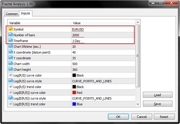
Also, pay attention to the Chart lifetime parameter setting the number of seconds, within which you are able to work with the utility. After clicking ОК, the analyzer appears in the upper left corner of the MetaTrader 5 main terminal window. The example is displayed on the below screenshot.
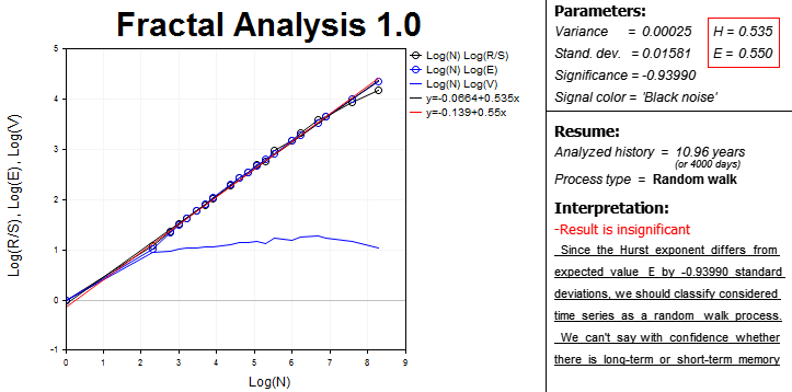
Eventually, all data and results necessary for the fractal analysis appear on the screen combined into blocks.
The left part features the area with graphical dependences on a logarithmic scale:
- R/S statistics from the number of observations in the sample;
- expected R/S statistics value E(R/S) of the number of observations;
- V statistics of the number of observations.
This is an interactive area involving the use of MetaTrader 5 chart analysis tools since it is sometimes quite difficult to define a cycle length without special means.
Curve and trend line equations are also present. Slopes of trend lines are used to define numerical Hurst exponents (H). Expected Hurst exponent (E) is calculated as well. These equations are in the right adjacent block. Dispersion, analysis significance and signal spectrum color are calculated there as well.
For convenience, the program calculates the length of the analyzed period in days. Keep that in mind, when evaluating the significance of the history data.
The "Process type" line specifies the time series parameter:
- persistent;
- anti-persistent;
- random walk.
Finally, the Interpretation block displays a brief summary that can be helpful for a novice in the field of the fractal analysis.
5.2. Operation example
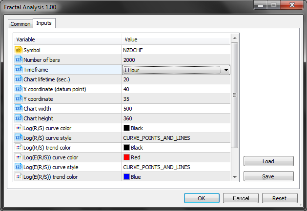
We should define what symbol and timeframe to use for analysis. Let's take NZDCHF and have a look at the last quotes on H1.
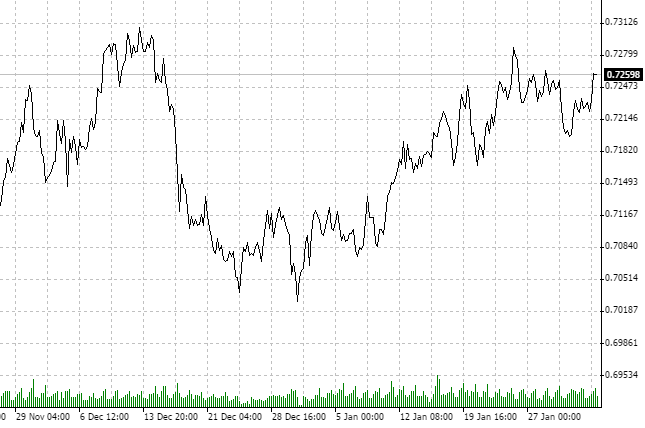
Please note that the market has been consolidating for about the last two months. Again, we are NOT interested in other investment horizons. It is quite possible that the D1 chart shows an up or downtred. We have selected H1 and a certain amount of history data.
Apparently, the process is anti-persistent. Let's check it using Fractal Analysis.
From 21.11 to 3.02, we have a 75-day history. After converting 75 days to hours, we receive 1800 hour data. Since there are not that many bars at the utility entry, specify the nearest value — 2000 analyzed hour periods.
The results are displayed below:
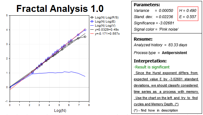
Thus, our hypothesis is confirmed, and the market demonstrates the considerable anti-persistent process on this horizon — the Hurst exponent H=0.490 which is almost three standard deviations lower than the expected value E=0.557.
Let's fix the result and use a slightly higher timeframe (H2) and accordingly twice smaller number of bars in history (1000 values). The results are as follows:
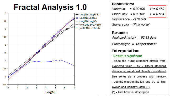
We see the anti-persistent process again. The Hurst exponent H=0.469 is more than three standard deviations lower than the expected exponent value E=0.564.
Now, let's try to find cycles.
We should return to the H1 chart and define the moment the R/S curve detaches from E(R/S). This moment is characterized by the formation of a top on V statistics graph. Thus, we are able to define the approximate cycle size.
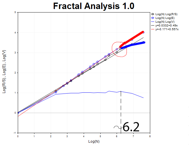
It is roughly equal to N1 = 2.71828^6.2 = 493 hours which is equivalent to 21 days.
Of course, a single experiment does not guarantee the reliability of its results. As mentioned above, it is necessary to try different timeframes and select all sorts of "timeframe — bar number" combinations to make sure the result is valid.
Let's perform a graphical analysis of 1000 H2 timeframe bars.
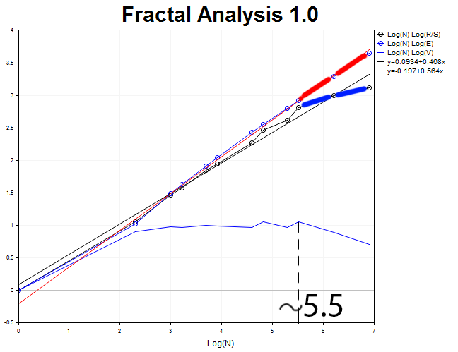
The cycle length is equal to N2 = 2.71828^5.5 = 245 two-hour periods (approximately, twenty days).
Now, let's analyze M30 timeframe and 4000 values. We obtain the anti-persistent process with the Hurst exponent H = 0.492 and the expected value E=0.55 exceeding H by 3.6 standard deviations.
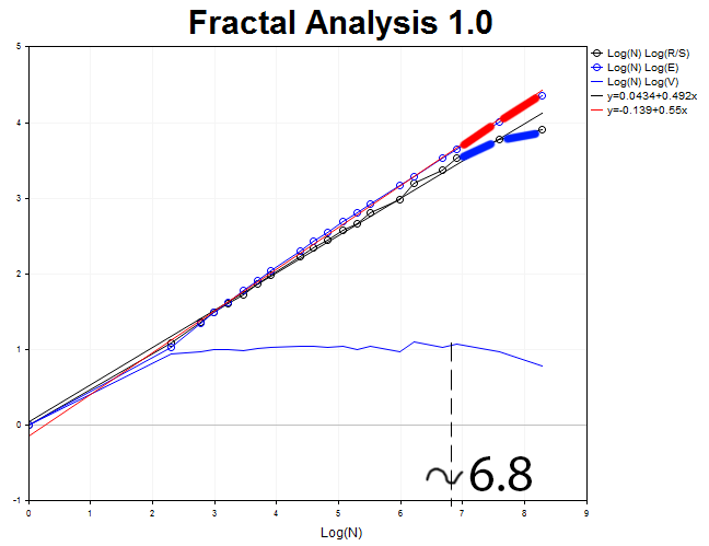
The cycle length N3 = 2.71828^6.8 = 898 thirty-minute segments (18.7 days).
Three tests are enough for a training example. Let's find the average value of the obtained period length M= (N1 + N2 + N3)/3 = (21 + 20 + 18.7)/3 = 19.9 (20 days).
As a result, we obtain the period, within which the technical data is reliable enough and can be used to develop a trading strategy. As I have already mentioned, the calculation and analysis provided above are meant for the investment horizon of two months. This means the analysis is not relevant for intraday trading since it probably features its own ultra-short cyclical processes, the presence or absence of which we have to prove. If the cycles are not detected, the technical analysis loses its relevance and efficiency. In that case, news trading and defining the market sentiments are the most reasonable solutions.
Conclusion
The fractal analysis is a certain synergy of technical, fundamental and statistical approach to forecasting the market dynamics. This is a versatile data processing method: R/S analysis and Hurst exponent are successfully used in geography, biology, physics and economics. The fractal analysis can be applied for developing scoring or estimation models applied by banks to analyze the solvency of borrowers.
As I have already said at the beginning of the article: In order to trade on Forex successfully, we need to know a bit more than other investors. Anticipating some misunderstanding here, I would like to warn the reader that the market tends to "deceive" the analyst. Therefore, be sure to check the presence of a non-periodic cycle on higher and lower timeframes at all times. If it is not detected on other timeframes, the cycle is most probably just a market noise.