Analysis of the Main Characteristics of Time Series
Victor | 17 January, 2012
Introduction
Analysis of processes represented by price series is a quite challenging task often requiring a significant amount of time and effort. It has to do with peculiarities of sequences under study as well as the fact that despite a great number of various publications it is sometimes difficult to find an adequate programming solution for a certain problem.
Even if a suitable script or indicator has been found, it does not mean that its source code would not need to be adjusted to the task at hand.
Furthermore, even for solution of simple problems, these programs may require the use of input parameters the point in which is well-known to developers but is not always completely clear to a user.
These difficulties certainly cannot become an insuperable obstacle in serious research but when one wants to prove an assumption or simply satisfy one's curiosity, such curiosity will more often than not remain unsatisfied. That is why I had an idea to create a universal programming tool allowing for easy preliminary analysis of the main characteristics and parameters of an input sequence.
Such a tool should be utterly simple in its installation without requiring any input parameters to maximally simplify its use. At the same time, the estimated parameters and characteristics should adequately and clearly reflect the nature of the sequence under consideration.
Preliminary estimate of characteristics could help determine the ways for further in-depth study or reject any given assumption at an early stage and avoid the time loss with regard to further study.
It is well-known that universal software is often poorly compared to customized software in terms of its characteristics. This is a regular price for universality which is almost always achieved by means of the entire system of compromises. This article however represents an effort to create a universal tool that allows to maximally facilitate the preliminary analysis of characteristics of sequences.
Installation and Capacity
TSAnalysis.zip file which can be found at the end of the article includes \TSAnalysis directory containing all files required for work. After unzipping, the directory with all its contents (without renaming it) should be copied into \MQL5\Scripts directory. The copied directory \TSAnalysis contains a test script TSAexample.mq5 which can be run after compiling.
This script shall prepare data and call the default browser to display it using TSAnalysis class. It should be noted that the use of external DLLs shall be enabled in the Terminal for the normal operation of TSAnalysis class. To uninstall, it is sufficient to simply delete \TSAnalysis directory.
The entire source code which is used for analysis of sequences is represented by TSAnalysis class and can be found only in TSAnalysis.mqh file.
When using this class for an input sequence, it estimates and can display the following information:
- Number of elements in the sequence;
- Maximum and minimum value of the sequence (max, min);
- Median;
- Mean;
- Variance;
- Standard deviation;
- Unbiased variance;
- Unbiased standard deviation;
- Skewness;
- Kurtosis;
- Excess kurtosis;
- Jarque-Bera test;
- Jarque-Bera test p-value;
- Adjusted Jarque-Bera test;
- Adjusted Jarque-Bera test p-values;
- Limits for values not belonging to the given sequence (outliers);
- Histogram data;
- Normal Probability Plot data;
- Correlogram data;
- 95% confidence bands for autocorrelation function;
- Data of the Spectral Plot calculated via the autocorrelation function;
- Partial Autocorrelation Function Plot data;
- Data of the Spectral Estimation Plot calculated using maximum entropy method.
In order to visually display the obtained results in TSAnalysis class under consideration, a virtual show method is used that is in charge of a pre-prepared information display method only.
Therefore by redefining this method in TSAnalysis class descendants, one can arrange for the output of results in any way possible, not only by using an HTML file as in the base class where, upon generation of a data file for displaying charts, a web browser is called.
Before proceeding to the TSAnalysis class review, we will illustrate the result of its use through a test sequence of data. The figure below shows the TSAexample.mq5 script operating result.

Figure 1. TSAexample.mq5 script operating result
After a brief familiarization with the TSAnalysis class capacity, we will now move to a more detailed consideration of the class itself.
TSAnalysis Class
TSAnalysis class (see TSAnalysis.mqh) includes only one available (public) method Calc which is in charge of all necessary calculations following which the virtual method show is called. The show method will be briefly reviewed later on, and we will now proceed to a step-to-step clarification of the main point of the calculations made.
When using TSAnalysis class, some constraints are imposed on the input sequence under study.
First, the sequence shall consist of at least eight elements. Such a constraint is probably not very rigid as it will hardly be necessary to study such short sequences for practical purposes.
In addition to the minimum sequence length constraint, the input sequence variance value is required to be other than near zero. This requirement is due to the fact that the variance value is used in further calculations and cannot be less than a certain value for a stable result.
Sequences with a very low variance value are not so common so this constraint will probably not be a serious disadvantage either. Where the sequence is too short and where there is a near-zero variance value, the calculations will be interrupted and a relevant error message will appear in the log.
There is yet another implicit constraint with regard to the maximum allowed length of an input sequence. This constraint is not explicitly set and depends on the performance of a computer in use and its memory capacity and is determined in a purely subjective way by the time required for the script execution and the speed of drawing results in a web browser. It is assumed that processing of sequences consisting of 2-3 thousand elements should not cause serious difficulties.
The calculation of statistical parameters of the sequence will be based on the below fragment of the Calc method source code (see TSAnalysis.mqh).
The description of the employed algorithm can be found by following this link "Algorithms for Calculating Variance".
. . .
Mean=0; sum2=0; sum3=0; sum4=0;
for(i=0;i<NumTS;i++)
  {
  n=i+1; delta=TS[i]-Mean;
  a=delta/n; Mean+=a;                                       // Mean (average)
  sum4+=a*(a*a*delta*i*(n*(n-3.0)+3.0)+6.0*a*sum2-4.0*sum3); // sum of fourth degree
  b=TS[i]-Mean;
  sum3+=a*(b*delta*(n-2.0)-3.0*sum2);                       // sum of third degree
  sum2+=delta*b;                                            // sum of second degree
  }
. . .
As a result of execution of this fragment, the following values are calculated
![]()
where n = NumTS is the number of elements in the sequence.
Using the obtained values, we calculate the following parameters.
Variance and standard deviation:
![]()
Unbiased variance and standard deviation:
![]()
Skewness:
![]()
Kurtosis. Minimum kurtosis is 1, kurtosis of the normally distributed sequence will be 3.
![]()
Excess kurtosis:
![]()
In this case the minimum kurtosis is -2, and kurtosis of the normally distributed sequence will be 0.
Conventionally, when performing the first preliminary goodness-of-fit test on a sequence, the Jarque-Bera statistic is used which is easily calculated using the known values of skewness and kurtosis. Statistical significance (p-value) for the Jarque-Bera statistic, upon the increase of the sequence length, is asymptotically tending to the inverse chi-squared distribution function with two degrees of freedom.
Thus,
![]()
Where the sequence is short, the p-value obtained in this manner is bound to have an appreciable error. This very calculation option is nevertheless very often used. It is hard to say why - perhaps it has to do with simple and clear formulas used or it could be the fact that the Jarque-Bera statistic in itself does not represent an ideal goodness-of-fit test and therefore there is no point in more accurate calculations.
In our case the Jarque-Bera statistic and the relevant p-value are calculated in the Calc method (TSAnalysis.mqh) in accordance with the above formulas.
Besides, an adjusted Jarque-Bera test is calculated additionally:
![]()
where
![]()
The adjusted version of the Jarque-Bera test for short sequences reduces the error of the p-value calculated in the specified manner but does not fully eliminate it.
The final result of the analysis is supposed to include an input sequence chart displaying the line corresponding to the mean and the lines defining the limits outside of which the values can be considered invalid and not belonging to the given sequence (outliers).
These limits are in this case calculated as follows:
![]()
![]()
This formula is provided in the book by S. V. Bulashev "Statistics for Traders" with a reference to the book by P. V. Novitsky and I.A. Zograf "Estimation of Error in Measurement Results". After determining the limits, no processing of the input sequence is intended; the limits are supposed to be displayed for information only.
In addition to the input sequence chart, a histogram reflecting an empirical estimate of the input sequence distribution is intended to be displayed. The number of intervals for the histogram is defined as follows (S. V. Bulashev "Statistics for Traders"):
![]()
The result is rounded down to the nearest odd integer value. If the obtained value is less than five, the value of 5 is used.
The number of elements in data arrays for X-axis and Y-axis of the histogram corresponds to the obtained number of intervals plus two, since a zero value column is added to the left and right of the histogram.
A fragment of the code (see TSAnalysis.mqh) preparing the data for building a histogram is set forth below.
. . .
n=(int)MathRound((Kurt+1.5)*MathPow(NumTS,0.4)/6.0);
if((n&0x01)==0)n--; if(n<5)n=5;                         // Number of bins
ArrayResize(XHist,n);
ArrayResize(YHist,n);
ArrayInitialize(YHist,0.0);
a=MathAbs(TSort[0]-Mean); b=MathAbs(TSort[NumTS-1]-Mean);
if(a<b)a=b; v=Mean-a;
delta=2.0*a/n;
for(i=0;i<n;i++)XHist[i]=(v+(i+0.5)*delta-Mean)/StDev; // Histogram. X-axis
for(i=0;i<NumTS;i++)
  {
  k=(int)((TS[i]-v)/delta);
  if(k>(n-1))k=n-1;
  YHist[k]++;
  }
for(i=0;i<n;i++)YHist[i]=YHist[i]/NumTS/delta*StDev;   // Histogram. Y-axis
. . .
In the above code:
- NumTS is the number of elements in the sequence,
- XHist[] and YHist[] are arrays containing values for X- and Y-axis, respectively,
- TSort[] is the array containing a sorted input sequence.
Using this calculation method, X-axis values will be expressed in standard deviation units and Y-axis values will correspond to the probability density.
For purposes of building a chart with the normal distribution axis, the input sequence sorted in ascending order is used as Y-axis values. The number of Y- and X-axis values is supposed to be equal. In order to calculate the X-axis values, one first has to find the median values as in the uniform distribution law:
![]()
![]()
![]()
They are further used to calculate the X-axis values by means of the inverse normal distribution function (see ndtri method).
In order to create an autocorrelation function (ACF) plot, partial autocorrelation function (PACF) plot and calculate the spectral estimate using the maximum entropy method, the autocorrelation function values should be found for the input sequence.
We will define the number of values that are supposed to be displayed on ACF and PACF plots as follows:
![]()
![]()
![]()
The number of values determined in the specified manner will be quite sufficient for display of the autocorrelation function on the plot but for further calculation of spectral estimate it is advisable to have a greater number of calculated ACF values which in our case will be equal to the order of the autoregressive model employed.
The IP model order will be defined by the obtained NLags value:
![]()
![]()
It is quite difficult to formalize the process of determining the optimal order of the model for spectral estimation. A low-order model will bring extremely smoothed results while a high-order model will most likely lead to an unstable spectral estimate with a large range of values.
Besides, the model order is also affected by the nature of the input sequence, therefore the IP order determined using the above formula will in some cases be too high and in other cases too low. Unfortunately, an effective approach to determining the required model order has not been found.
Thus, for the input sequence one should determine the number of the ACF values equal to the IP model order which is used for the spectral estimation of the sequence.
. . .
ArrayResize(cor,IP);
a=0;
for(i=0;i<NumTS;i++)a+=TSCenter[i]*TSCenter[i];
for(i=1;i<=IP;i++)
  {
  c=0;
  for(k=i;k<NumTS;k++)c+=TSCenter[k]*TSCenter[k-i];
  cor[i-1]=c/a;                                   // Autocorrelation
  }
. . .
This fragment of the source code (see TSAnalysis.mqh) illustrates the process of calculating the autocorrelation function (ACF). The calculation result is placed in cor[] array. As can be seen, a zero autocorrelation coefficient is calculated first, followed by the calculation and normalization of the remaining coefficients in the loop. Upon such normalization, the zero coefficient will always be equal to one so there is no need in saving it in cor[] array.
This array contains the number of coefficients equal to IP starting from the first one. When calculating the ACF, TSCenter[] array is used; it contains the input sequence of the elements from all of which the mean value was subtracted.
In order to reduce the time required for calculating the ACF, one can make use of the methods employing fast transformation algorithms, e.g. FFT. But in this case the time required for calculating the ACF is quite acceptable so there is probably no need in complicating the programming code.
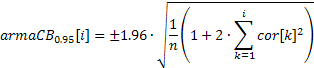
An ACF plot (correlogram) can easily be built using the obtained values of the correlation coefficients. In order to be able to display the 95% confidence bands on this plot, their values can be calculated using the below formulas.
For the bands used to test for randomness:
![]()
For the bands used to determine the ARIMA model order:
The value of the confidence band in the first case will be constant and will be increasing with the increase of the autocorrelation coefficient in the second case.
A very smoothed frequency response of the input sequence reflecting only the general trend of the frequency distribution may sometimes be of interest. For example, considerable rises in low- or high-frequency range, predominance of mid-range frequencies, etc.
It is advisable to display such frequency response in linear scale to strongly emphasize the dominant frequency ranges. Such amplitude-frequency response (AFR) can be plotted based on the previously obtained autocorrelation coefficients. For calculation of the AFR we will use the number of coefficients equal to the number displayed on the ACF plot.
Given that this number is not big, the spectral estimates obtained as a result should be quite smooth.
The frequency response of the sequence in this case can be expressed by means of autocorrelation coefficients as follows:
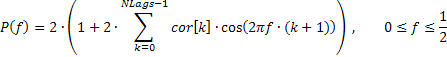
A fragment of the code (see TSAnalysis.mqh) which is used to calculate the AFR based on the provided formula, is set forth below
. . .
n=320;                                              // Number of X-points
ArrayResize(Spect,n);
v=M_PI/n;
for(i=0;i<n;i++)
  {
  a=i*v; b=0;
  for(k=0;k<NLags;k++)b+=((double)NLags-k)/(NLags+1.0)*ACF[k]*MathCos(a*(k+1));
  Spect[i]=2.0*(1+2*b);                             // Spectrum Y-axis
  }
. . .
It should be noted that the correlation coefficient values in the above code are, for further smoothing, multiplied by the triangular window function.
For a more detailed spectral analysis, the maximum entropy method was selected as another compromise. Selection of a universal spectral estimation method is quite difficult. Disadvantages associated with classical non-parametric methods of spectral analysis are well known.
Periodogram and correlogram methods can serve as examples of such methods that are easily implemented using fast Fourier transform algorithms. But despite the high stability of the results, these methods require very long input sequences in order to get an adequate resolution power. In contrast, parametric methods of spectral estimation (e.g. autoregressive methods) can ensure much higher resolution for short sequences.
Unfortunately, when using them, one has to take into consideration not only peculiarities of a certain implementation of these methods but also the nature of the input sequence. At the same time it is quite difficult to determine the optimal AR model order the increase in which leads to increasing resolution power but scattered results obtained. If very high-order models are used, these methods start giving unstable results.
Comparative characteristics of different spectral estimation algorithms can be found in the book by S. L. Marple "Digital Spectral Analysis with Applications". As already mentioned, the maximum entropy method was selected in this case. This method results in probably the lowest resolution power as compared to other autoregressive methods but it has been selected with a view to obtaining more stable spectral estimates.
Let us have a look at the order of autoregressive spectral estimate calculations. The choice of the model order was touched upon earlier so we will assume that the model order has already been selected being equal to IP and the IP autocorrelation coefficients cor[] have been calculated.
In order to obtain the autoregressive coefficients using the known autocorrelation coefficients, the Levinson-Durbin algorithm is used implemented as the LevinsonRecursion method.
//-----------------------------------------------------------------------------------
// Calculate the Levinson-Durbin recursion for the autocorrelation sequence R[]
// and return the autoregression coefficients A[] and partial autocorrelation
// coefficients K[]
//-----------------------------------------------------------------------------------
void TSAnalysis::LevinsonRecursion(const double &R[],double &A[],double &K[])
  {
  int p,i,m;
  double km,Em,Am1[],err;

  p=ArraySize(R);
  ArrayResize(Am1,p);
  ArrayInitialize(Am1,0);
  ArrayInitialize(A,0);
  ArrayInitialize(K,0);
  km=0;
  Em=1;
  for(m=0;m<p;m++)
    {
    err=0;
    for(i=0;i<m;i++)err+=Am1[i]*R[m-i-1];
    km=(R[m]-err)/Em;
    K[m]=km; A[m]=km;
    for(i=0;i<m;i++)A[i]=(Am1[i]-km*Am1[m-i-1]);
    Em=(1-km*km)*Em;
    ArrayCopy(Am1,A);
    }
  return;
  }
The method has three input parameters. All three parameters are references to arrays. When calling this method, the input autocorrelation coefficients should be placed in the first array R[]. In the course of calculations these values remain unchanged.
The obtained autocorrelation coefficients will be placed in array A[]. Besides that, array K[] will contain partial autocorrelation function values equal to autoregressive model reflection coefficients taken with opposite sign. The model order is not passed as an input parameter; it is assumed to be equal to the number of elements in the input array R[].
The output array sizes are therefore required to be not less than the input array size; fulfillment of this requirement is not checked inside the function. Upon completion of the calculations, the zero autoregressive coefficient and zero coefficient of the partial autocorrelation function are not saved in arrays A[] and K[].
It is assumed that they are always equal to one. Thus, the output arrays will, as in the input sequence, contain coefficients with indices from 1 to IP (not to be confused with array indices which start from 0).
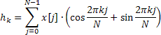
The obtained values of the partial autocorrelation function are further used only for display on a respective plot, and autoregressive coefficients serve as the basis for calculation of the frequency response estimate which is defined by the following formula:
![]()
Frequency response is calculated for 4096 normalized frequency values over the range from 0 to 0.5. Direct calculation of the AFR values using the above formula takes too much time which can be substantially reduced by using the fast Fourier transform algorithm for calculating the sum of complex exponentials.
For this purpose, Calc method employs the fast Hartley transform (FHT) instead of the fast Fourier transform.
The Hartley transform does not involve complex operations and both the input and output sequences are valid. The inverse Hartley transform is calculated using the same formula only requiring an additional factor 1/N.
In a valid input sequence, there is a simple connection between the coefficients of this transform and the coefficients of the Fourier transform
![]()
Information on the fast Hartley transform algorithms can be found here "FXT algorithm library" and "Discrete Fourier and Hartley Transforms".
In the given implementation, the fast Hartley transform function is represented by fht method.
//-----------------------------------------------------------------------------------
// Radix-2 decimation in frequency (DIF) fast Hartley transform (FHT).
// Length is N = 2 ** ldn
//-----------------------------------------------------------------------------------
void TSAnalysis::fht(double &f[], ulong ldn)
  {
  const ulong n = ((ulong)1<<ldn);
  for (ulong ldm=ldn; ldm>=1; --ldm)
    {
    const ulong m = ((ulong)1<<ldm);
    const ulong mh = (m>>1);
    const ulong m4 = (mh>>1);
    const double phi0 = M_PI / (double)mh;
    for (ulong r=0; r<n; r+=m)
      {
      for (ulong j=0; j<mh; ++j)
        {
        ulong t1 = r+j;
        ulong t2 = t1+mh;
        double u = f[t1];
        double v = f[t2];
        f[t1] = u + v;
        f[t2] = u - v;
        }
      double ph = 0.0;
      for (ulong j=1; j<m4; ++j)
        {
        ulong k = mh-j;
        ph += phi0;
        double s=MathSin(ph);
        double c=MathCos(ph);
        ulong t1 = r+mh+j;
        ulong t2 = r+mh+k;
        double pj = f[t1];
        double pk = f[t2];
        f[t1] = pj * c + pk * s;
        f[t2] = pj * s - pk * c;
        }
      }
    }
  if(n>2)
    {
    ulong r = 0;
    for (ulong i=1; i<n; i++)
      {
      ulong k = n;
      do {k = k>>1; r = r^k;} while ((r & k)==0);
      if (r>i) {double tmp = f[i]; f[i] = f[r]; f[r] = tmp;}
      }
    }
  }
When calling this method, a reference to the input data array f[] and the unsigned integer ldn defining the transform length N = 2 ** ldn are passed in input . The size of array f[] should be not less than the transform length N. Bear in mind that there are no checks for this inside the function. Also remember that the transform result is stored in the array where the input data was placed.
Following the transform, the input data itself is not stored. In Calc method under consideration, a transform of length N=8192 is used in order to calculate 4096 AFR values. Following the calculation of the transform squared magnitude and taking the reciprocal, the obtained result is normalized to its maximum value and logarithmically scaled.
Other than that, there are no major peculiarities of Calc method; if necessary, one can have a closer look at its implementation by referring to TSAnalysis.mqh.
All the values obtained and prepared for display as a result of the calculations are saved in variables being the members of the TSAnalysis class. Therefore, they do not have to be passed as arguments when calling the virtual method show in order to display the results.
Visualization
As already mentioned, the show method is declared as virtual. So, by redefining it, one can implement the required method for displaying the calculation results that would be different from the proposed one. Visualization in the proposed TSAnalysis class is carried out by means of data file preparation and calling a web browser for display of the data.
In order for a web browser to be able to display such data, TSA.htm file is used located in the same directory as the rest of the project files. This method for displaying graphical information was earlier described in the article "Graphs and Diagrams in HTML".
TSAnalysis class of the show method is in charge of formatting and saving all calculation results intended for display into a string-type variable (see TSAnalysis.mqh). A long line generated in this manner is saved into TSDat.txt in a single step. Creation of this file and saving of data into it is carried out using the standard MQL5 tools therefore the file is created in \MQL5\Files directory.
This file is then moved to the directory of this project by calling the external system functions. This is followed by a call of a web browser displaying TSA.htm that uses data from TSDat.txt. Since the system functions are called in the show method, the use of external DLLs shall be enabled in the Terminal for working with TSAnalysis class.
Examples
TSAexample.mq5 included in TSAnalysis.zip archive is an example of using TSAnalysis class.
//-----------------------------------------------------------------------------------
//                                                                     TSAexample.mqh
//                                                                      2011, victorg
//                                                                https://www.mql5.com
//-----------------------------------------------------------------------------------
#property copyright "2011, victorg"
#property link      "https://www.mql5.com"

#include "TSAnalysis.mqh"
//-----------------------------------------------------------------------------------
// Script program start function
//-----------------------------------------------------------------------------------
void OnStart()
  {
  double bd[]={47,64,23,71,38,64,55,41,59,48,71,35,57,40,58,44,80,55,37,74,51,57,50,
  60,45,57,50,45,25,59,50,71,56,74,50,58,45,54,36,54,48,55,45,57,50,62,44,64,43,52,
  38,59,55,41,53,49,34,35,54,45,68,38,50,60,39,59,40,57,54,23};

  TSAnalysis *tsa=new TSAnalysis;

  tsa.Calc(bd);

  delete tsa;

  }
As can be seen, the reference to the class is fairly simple; if there is a prepared array containing the input sequence, it will not take a lot of effort to pass it to Calc method for analysis. In addition, you should remember to free up the memory by calling delete. The result of running this script has already been provided at the beginning of the article.
In order to demonstrate the efficiency of the spectral estimates produced, let us turn to additional examples where generated sequences will be used.
For a start, we will use a sequence consisting of two sinusoids.
int i,n;
double a,x[];

n=400;
ArrayResize(x,n);
a=2*M_PI;
for(i=0;i<n;i++)x[i]=MathSin(0.064*a*i)+MathSin(0.071*a*i);
The figure below demonstrates the frequency response estimate of this sequence.

Figure 2. Spectral estimation. Two sinusoids
Although both sinusoids are well observable, zooming in on the chart area of interest allowed us to discover that the peaks are located at frequencies of 0.0637 and 0.0712. In other words, they are somewhat different from the true values. Where a sequence consists of a single sinusoid, such bias of an estimate is not observed. Let us consider this occurrence to be the effect of the selected method of spectral analysis.
We will further complicate the task by adding a random component to our sequence. For this purpose, a pseudo-random sequence generator will be used represented by RNDXor128 class that can be found in the RNDXor128.zip archive at the end of the article.
The below code fragment was used to generate a test signal.
int i,n;
double a,x[];

RNDXor128 *rnd=new RNDXor128;
n=800;
ArrayResize(x,n);
a=2*M_PI;
for(i=0;i<n;i++)x[i]=MathSin(0.064*a*i)+MathSin(0.071*a*i)+rnd.Rand_Norm();
delete rnd;
In this example, a random signal with normal distribution and unit variance was added to two sinusoids.
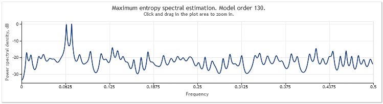
Figure 3. Spectral estimation. Two sinusoids plus a random signal
In this case, the sinusoidal components remain well discernible.
A five-fold increase in amplitude of the random component results in substantially masked sinusoids.
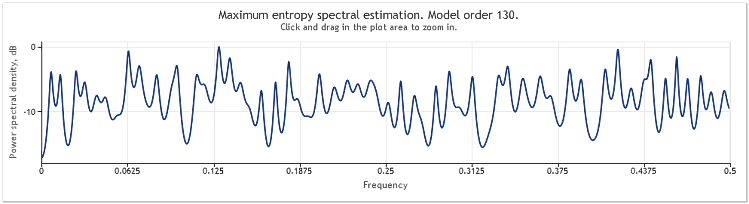
Figure 4. Spectral estimation. Two sinusoids plus a random signal with larger amplitude
When the sequence length is increased from 400 to 800 elements, the sinusoids become well observable again.
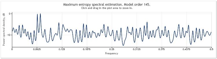
Figure 5. Two sinusoids plus a random signal with larger amplitude. N=800
The autoregressive model order has thereby increased from 130 to 145. Increase in the sequence length led to higher order of the model and as a result the resolution power of the spectral estimate increased - the chart peaks became markedly sharper.
Spectral estimation of the quotes for EURUSD, D1 over two years (2009 and 2010) can be shown as follows.
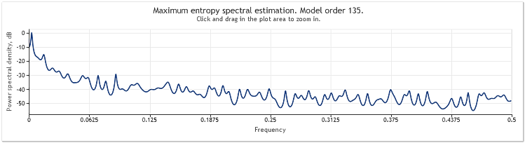
Figure 6. EURUSD quotes. 2009-2010. Period D1
The input sequence consisted of 519 values and the model order, as follows from the figure, appeared to be 135.
As can be seen, this spectral estimate contains a number of distinct peaks. But this estimation alone is not sufficient for determining whether these peaks are periodic components of the quotes.
Occurrence of peaks in frequency response can be caused by a high-level random component present in the quotes or by explicit non-stationarity of the sequence in question.
It is therefore always advisable to verify the obtained result using the data from another fraction of the sequence or another time frame before drawing a final conclusion regarding the presence of the periodic component. Besides, when studying cyclic recurrence, one can try using the sequence differences instead of the sequence itself.
Conclusion
Since the method of spectral estimation employed in the article is based on autocorrelation coefficients, the mean of the input sequence always appears to be deleted from the sequence upon application of the method. It is often absolutely necessary to delete a constant component from the input sequence but, when using autoregressive methods, such deletion can, in some cases, cause distortion of the spectral estimate in the low-frequency range.
An example of such distortions is set forth at the end of chapter "Summary of Results Regarding Spectral Estimates" in the book by S. L. Marple "Digital Spectral Analysis with Applications". In our case, the method of spectral analysis employed leaves us no other choice so simply bear in mind that spectral estimation is always carried out with respect to a sequence with a deleted mean.
References
- Wuertz, Diethelm and Katzgraber, Helmut (2009): Precise finite-sample quantiles of the Jarque-Bera adjusted Lagrange multiplier test, Swiss Federal Institute of Technology, Zurich,2009.
- Tanweer-ul-Islam, Asad Zaman, Normality Testing - A new Direction, IIE, International Islamic University, Islamabad, Pakistan, 2008.
- Carlos M. Urzua, Portable and powerful tests for normality, Tecnologico de Monterrey, Campus Ciudad de Mexico, 2007.
- Comparison of Common Tests for Normality
- S. V. Bulashev. Statistics for Traders. - М.: Kompania Sputnik +, 2003. - 245 pp.
- P. V. Novitsky, I. A. Zograf. Estimation of Error in Measurement Results. Energoatomizdat, 1991.
- S. L. Marple, Jr. Digital Spectral Analysis with Applications. Moscow: Mir, 1990.
- David J. Sheskin, Handbook of Parametric and Nonparametric Statistical Procedures, Chapman and Hall/CRC.