Visualize this! MQL5 graphics library similar to 'plot' of R language

MetaQuotes | 23 March, 2017

When studying trading logic, visual representation in the form of graphs is of great importance. A number of programming languages popular among the scientific community (such as R and Python) feature the special 'plot' function used for visualization. It allows drawing lines, point distributions and histograms to visualize patterns.

The important advantage of the 'plot' function is that you need only a few lines of code to plot any graph. Simply pass the data array as a parameter, specify the graph type and you are ready to go! The 'plot' function performs all the routine operations of calculating a scale, building axes, selecting a color, etc.

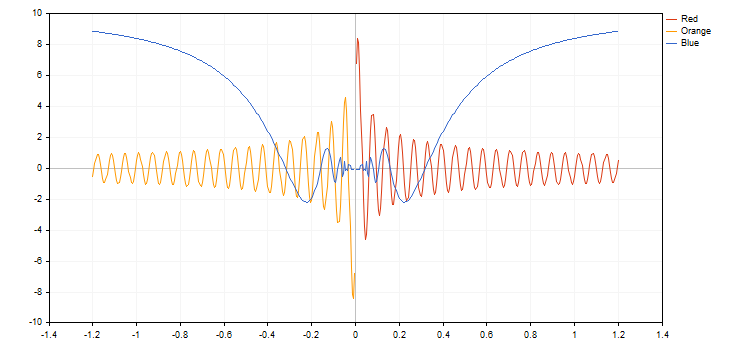
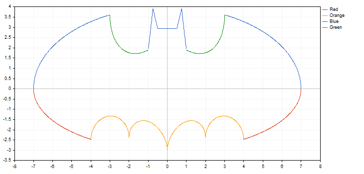
In MQL5, all features of the function are represented by the graphics library method from the Standard Library. The sample code and the result of its execution are shown below:

CCanvas base class and its development

The standard library contains the CCanvas base class designed for fast and convenient plotting of images directly on price charts. The class is based on creating a graphical resource and plotting simple primitives (dots, straight lines and polylines, circles, triangles and polygons) on the canvas. The class implements the functions for filling shapes and displaying text using the necessary font, color and size.

Initially, CCanvas contained only two modes of displaying graphical primitives — with antialiasing (AA) and without it. Then, the new functions were added for plotting the primitives based on the Wu's algorithm:

• LineWu — straight line
• PolylineWu — polyline
  
• PolygonWu — polygon
  
• TriangleWu — triangle
  
• CircleWu — circle
• EllipseWu — ellipse

The Wu's algorithm combines high-quality elimination of aliasing with the operation speed close to the Bresenham's algorithm one without anti-aliasing. It also visually differs from the standard anti-aliasing algorithm (AA) implemented in CCanvas. Below is an example of plotting a circle using three different functions:

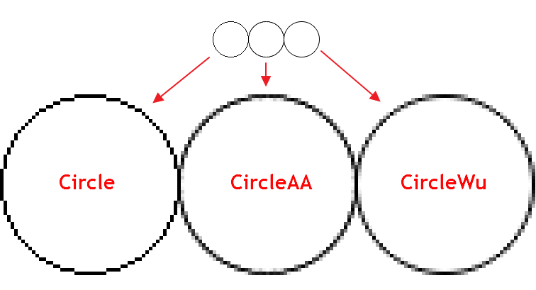
As we can see, CircleAA() with the standard smoothing algorithm draws a thicker line as compared to the CircleWu() function according to the Wu's algorithm. Due to its smaller thickness and better calculation of transitional shades, CircleWu looks more neat and natural.

There are also other improvements in the CCanvas class:

1. Added the new ellipse primitive with two anti-aliasing options — EllipseAA() and EllipseWu()
   
2. Added the filling area function overload with the new parameter responsible for the "filling sensitivity" (the threshould parameter).

The algorithm of working with the library

1. After connecting the library, we should create the CGraphic class object. The curves to be drawn will be added to it.

Next, we should call the Create() method for the created object. The method contains the main graph parameters:

1. Graph ID
2. Object name
3. Window index
   
4. Graph anchor point
5. Graph width and height

The method applies the defined parameters to create a chart object and a graphical resource to be used when plotting a graph.

As a result, we have a ready-made canvas.

2. Now, let's fill our object with curves. Adding is performed using the CurveAdd() method able to plot curves in four different ways:

1. Based on the double type one-dimensional array. In this case, values from the array are displayed on Y axis, while array indices serve as X coordinates.
2. Based on two x[] and y[] double type arrays.
3. Based on the CPoint2D array.
4. Based on the CurveFunction() pointer and three values for building the function arguments: initial, final and increment by argument.

The CurveAdd() method returns the pointer to the CCurve class providing fast access to the newly created curve and ability to change its properties.

3. Any of the added curves can then be displayed on the chart. This can be done in three ways.

1. By using the CurvePlotAll() method that automatically draws all curves added to the chart.
   graphic.CurvePlotAll();
2. By using the CurvePlot() method that draws a curve by the specified index.
   graphic.CurvePlot(0);
3. By using the Redraw() method and setting the curve's Visible property to 'true'.
   curve.Visible(true);
   graphic.Redraw();

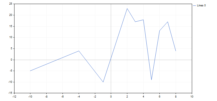
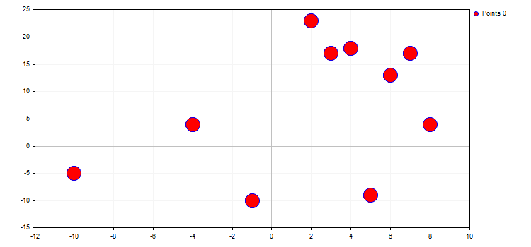
4. In order to plot a graph on the chart, call the Update() method. As a result, we obtain the entire code of the script for plotting a simple graph:

Below is the resulting graph:

The properties of the graph and any of its functions can be changed at any moment. For example, we can add labels to the graph axes, change the name of the curve and enable the mode of spline approximation for it:

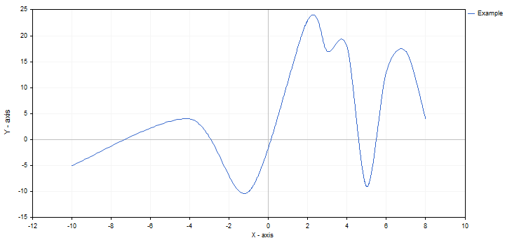
If the changes had been set after calling CurvePlotAll, we would have had to additionally call the Redraw method to see them.

Like many modern libraries, Graphics contains various ready-made algorithms considerably simplifying plotting charts:

1. The library is capable of auto generating contrasting colors of curves if they are not explicitly specified.
2. Graph axes feature the parametric auto scaling mode that can be disabled if necessary.
3. Curve names are generated automatically depending on their type and order of addition.
4. The graph's working area is automatically lined and actual axes are set.
5. It is possible to smooth curves when using lines.

The Graphics library also has a few additional methods for adding new elements to the chart:

1. TextAdd() — add a text to an arbitrary position on the chart. Coordinates should be set in real scale. Use the FontSet method for precise configuring of a displayed text.
   
2. LineAdd() — add a line to an arbitrary position on the chart. Coordinates should be set in real scale.
3. MarksToAxisAdd() — add new labels to a specified coordinate axis.

Data on adding the elements is not stored anywhere. After plotting a new curve on the chart or re-drawing a previous one, they disappear.

Graph types

The Graphics library supports basic types of curves plotting types. All of them are specified in the ENUM_CURVE_TYPE enumeration:

1. CURVE_POINTS — draw a point curve
2. CURVE_LINES — draw a line curve
3. CURVE_POINTS_AND_LINES — draw both point and line curves
4. CURVE_STEPS — draw a stepped curve
   
5. CURVE_HISTOGRAM — draw a histogram curve
6. CURVE_NONE — do not draw a curve
   

Each of these modes has its own properties affecting the display of a curve on the chart. The CCurve pointer to a curve allows fast modification of these properties. Therefore, it is recommended to remember all the pointers returned by the CurveAdd method. A property name always starts with a curve drawing mode it is used in.

Let's have a more detailed look at the properties of each of the types.

1. CURVE_POINTS is the fastest and simplest mode. Each curve coordinate is displayed as a point having specified properties:

• PointsSize — point size
• PointsFill — flag indicating if the filling is present
  
• PointsColor — filling color
  
• PointsType — points type
  

In this case, the color of the curve itself defines the color of the points' borders.

The type of points defines a certain geometric shape from the ENUM_POINT_TYPE enumeration. This shape is to be used for displaying all curve points. In total, ENUM_POINT_TYPE includes ten main geometric shapes:

1. POINT_CIRCLE — circle (used by default)
   
2. POINT_SQUARE — square
   
3. POINT_DIAMOND — diamond
   
4. POINT_TRIANGLE — triangle
   
5. POINT_TRIANGLE_DOWN — inverted triangle
   
6. POINT_X_CROSS — cross
   
7. POINT_PLUS — plus
   
8. POINT_STAR — star
   
9. POINT_HORIZONTAL_DASH — horizontal line
   
10. POINT_VERTICAL_DASH — vertical line
    

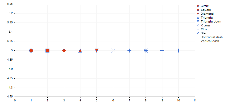
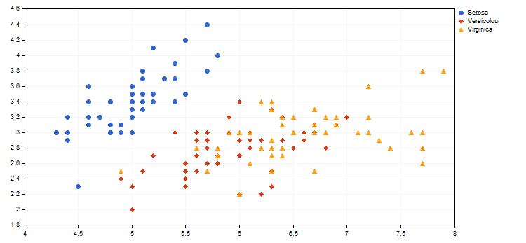
Below is an example of a visual representation of different kinds of iris (see the article "Using self-organizing feature maps (Kohonen Maps) in MetaTrader 5") from the attached IrisSample.mq5 script.

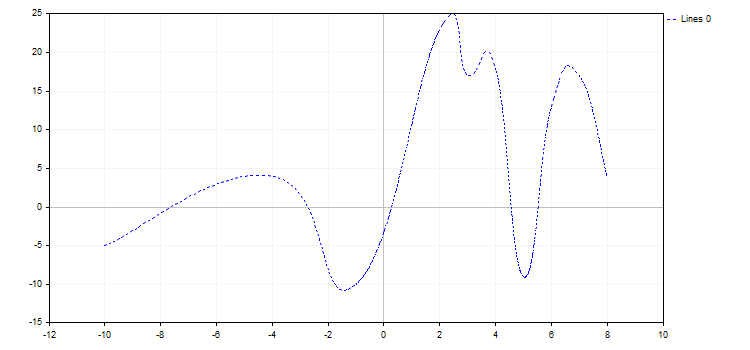
2. CURVE_LINES display mode is the main mode for visualizing the curves, in which each pair of dots is connected by one or several (in case of smoothing) straight lines. The mode properties are as follows:

• LinesStyle — line style from the ENUM_LINE_STYLE enumeration
• LinesSmooth — flag indicating if smoothing should be performed
  
• LinesSmoothTension — smoothing degree
  
• LinesSmoothStep — length of approximating lines when smoothing
  

Graphics features the standard parametric curve smoothing algorithm. It consists of two stages:

1. Two reference points are defined for each pair of points on the basis of their derivatives
2. A Bezier curve with a specified approximation step is plotted based on these four points

LinesSmoothTension parameter takes the values (0.0; 1.0]. If LinesSmoothTension is set to 0.0, no smoothing happens. By increasing this parameter, we receive more and more smoothed curve.

3. CURVE_POINTS_AND_LINES combines the previous two display modes and their properties.

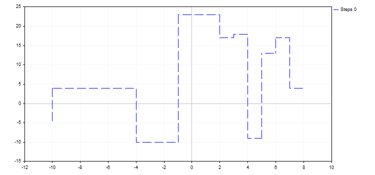
4. In the CURVE_STEPS mode, each pair of points is connected by two lines as a step. The mode has two properties:

• LinesStyle — this property is taken from CURVE_POINTS and defines the line style
• StepsDimension — step dimension: 0 — x (a horizontal line followed by a vertical one) or 1 — y (a vertical line followed by a horizontal one).
  

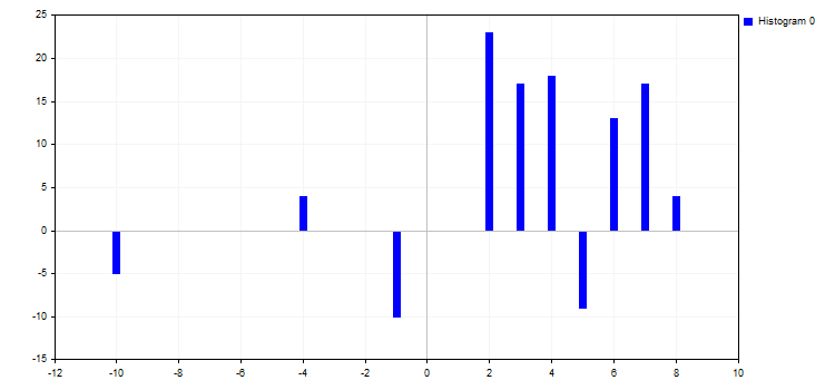
5. The CURVE_HISTOGRAM mode draws a standard bar histogram. The mode features a single property:

• HistogramWidth — bar width

If the value is too large, the bars may overlap, and the bars with greater Y value "absorb" the adjacent bars having smaller values.

6. The CURVE_NONE mode disables graphical representation of curves regardless of its visibility.

When auto scaling, all curves added to the chart have certain values. Therefore, even if the curve is not plotted or set to the CURVE_NONE mode, its values are still taken into account.

Graphs on functions — fast generation in a few lines

Another advantage of the library is working with CurveFunction pointers to functions. In MQL5, pointers to functions accept only global or static functions, while the function syntax should fully correspond to the pointer one. In our case, CurveFunction is configured for the functions receiving a double type parameter receiving double as well.

In order to construct a curve by a pointer to a function, we also need to accurately set the initial (from) and final (to) argument values, as well as its increment (step). The less the increment value, the more function points we have for constructing it. To create a data series, use CurveAdd(), while to plot a function, apply CurvePlot() or CurvePlotAll().

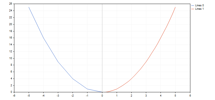
For example, let's create a parabolic function and draw it in various increments:

The library works with functions having break points (one of the coordinates has the value of plus or minus infinity or is non-numeric). Increment by function should be considered, since sometimes, we can simply miss a break point. In this case, a graph does not meet expectations. For example, let's draw two hyperbolic functions within the [-5.0; 5.0] segment with the first function having a step of 0.7 and the second one — 0.1. The result is displayed below:

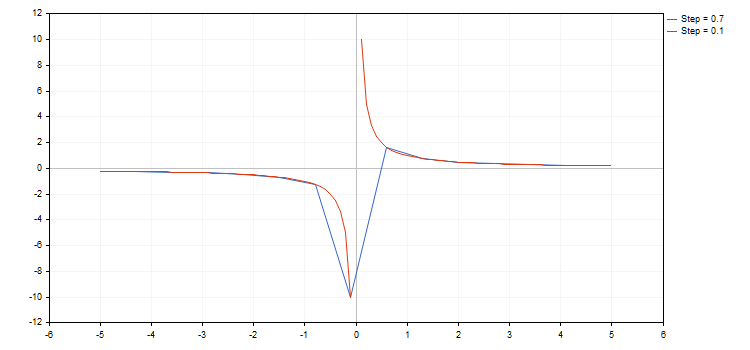
As we can see in the image above, we have simply missed the break point when using a step of 0.7. As a result, the resulting curve has almost nothing to do with the real hyperbolic function.

A zero divide error may occur when using the functions. There are two ways to handle this issue:

• disable the check for zero divide in metaeditor.ini
  
  [Experts]
  FpNoZeroCheckOnDivision=1
• or analyze an equation used in a function and return a valid value for such instances. An example of such handling using a macro can be found in the attached 3Functions.mq5 and bat.mq5 files.

  
  
  
  

  
  

Quick plotting functions

The Graphics library also includes a number of GraphPlot() global functions that perform all graph plotting stages based on available data and return an object name on the chart as a result. These functions are similar to 'plot' of R or Phyton languages allowing you to instantly visualize the data available in different formats.

The GraphPlot function has 10 various overloads allowing to plot a different number of curves on a single chart and set them in different ways. All you need to do is form data for plotting a curve using one of the available methods. For example, the source code for quick plotting of the x[] and y[] arrays looks as follows:

It looks similar on R:

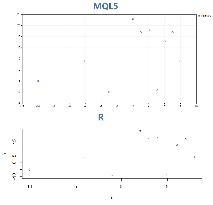
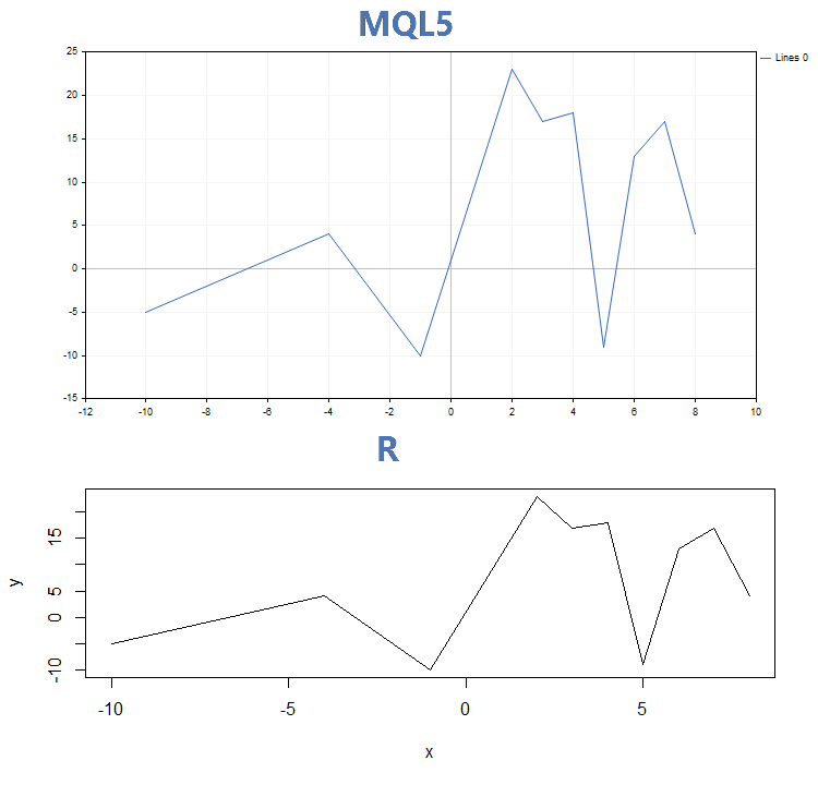
Results of comparing graphs by three main display modes built by the GraphPlot function on MQL5 and the plot function on R:

1. Point curves

2. Lines

3. Histogram

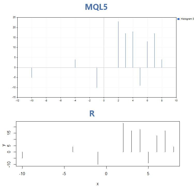
Apart from quite significant visual differences of the GraphPlot() and plot() functions operation, they apply different input parameters. While the plot() function allows setting specific curve parameters (for example, 'lwd' that changes the lines width), the GraphPlot() function includes only key parameters necessary for building data.

Let's name them:

1. Curve data in one of the four formats described above.
   
2. Plotting type (default is CURVE_POINTS).
   
3. Object name (default is NULL).

Each graph created using the Graphics library consists of a chart object and a graphical resource assigned to it. The graphical resource name is formed based on the object name by simply adding "::" before it. For example, if the object name is "SomeGraphic", the name of its graphical resource is "::SomeGraphic".

The GraphPlot() function has a fixed anchor point on a chart x=65 and y=45. The width and height of the graph are calculated based on the chart size: the width comprises 60% of the chart one, while the height is 65% of the chart's height. Thus, if the current chart dimensions are less than 65 to 45, the GraphPlot() function is not able to work correctly.

If you apply a name of an already created object while creating a graph, the Graphics library attempts to display the graph on that object after checking its resource type. If the resource type is OBJ_BITMAP_LABEL, plotting is performed on the same object-resource pair.

If an object name is explicitly passed to the GraphPlot() function, an attempt is made to find that object and display the graph on it. If the object is not found, a new object-resource pair is automatically created based on the specified name. When using the GraphPlot() function without an explicitly specified object name, the "Graphic" standard name is used. 

In this case, you are able to specify a graph anchor point and its size. To do this, create an object-resource pair with necessary parameters and pass the name of the created object to the GraphPlot() function. By creating a pair with the Graphic object name, we redefine and fix the standard canvas for the GraphPlot function eliminating the necessity to pass the object name at each call.

For example, let's take the data from the above example and set a new graph size of 750х350. Also, let's move the anchor point to the upper left corner:

Sample scientific graphs

The Standard Library includes the Statistics section featuring the functions for working with multiple statistical distributions from the probability theory. Each distribution is accompanied by a sample graph and a code to retrieve it. Here, we simply display these graphs in a single GIF. The source codes of examples are attached in the MQL5.zip file. Unpack them to MQL5\Scripts.

Key advantages of the graphics library

The MQL5 language allows developers not only to create trading robots and technical indicators but also perform complex mathematical calculations using the ALGLIB, Fuzzy and Statistics libraries. Obtained data is then easily visualized by provided graphics library. Most operations are automated, and the library offers the extensive functionality:

• 5 graph display types
• 10 chart marker types
  
• auto scaling of charts by X and Y axes
• color auto selection even if a graph features several constructions
  
• smoothing lines using the standard anti-aliasing or the more advanced Bresenham's algorithm
• ability to set spline approximation parameters for displaying lines
  
• ability to plot a graph using a single line of code based on the x[] and y[] arrays
• ability to plot graphs using pointers to functions
  

The graphics library simplifies plotting scientific graphs and raises the development of trading applications to a new level. The MetaTrader 5 platform allows you to perform mathematical calculations of any complexity and display results directly in the terminal window in a professional way.

Try the attached codes. You no more need third-party packages!