
Evaluation and selection of variables for machine learning models
Introduction
This article focuses on specifics of choice, preconditioning and evaluation of the input variables for use in machine learning models. Multiple methods of normalization and their features will be described here. Important moments of the process greatly influencing the final result of training models will also be revealed. We will have a closer look and evaluate new and little-known methods for determining the informativity and visualization of the input data.
With the "RandomUniformForests" package we will calculate and analyze the importance concept of a variable at different levels and in various combinations, the correspondence of predictors and a target, as well as the interaction between predictors, and the selection of an optimal set of predictors taking into account all aspects of importance.
With the "RoughSets" package we will look at the same issue of choosing predictors from a different angle and based on other concept. We will show that it's not only a set of predictors that can be optimal, a set of examples for training can also be optimized.
All calculations and experiments will be executed in the R language, to be specific - in Revolution R Open 3.2.1 .
1. Input variables (signs, predictors)
All variables, both input (independent, predictors) and output (target) may be of the following types:
Binary — has two values: {0,1}, {-1,1}, {"yes", "no"}, {"male", "female"}.
Nominal (factors) with a finite number of levels. For example, the factor "day of the week" has seven levels, and each of them can be named (Monday, Tuesday etc). Factors can be ordered and disordered. For example, the factor "hour of the day" has 24 levels and is ordered. The factor "district of a city" with 32 levels is disordered, since all levels are of equal importance. It should be explicitly specified, when declaring an ordered factor.
Quantitative (numerical) continuous. The range of continuous variables from Inf (infinity) to +Inf.
The "raw" data quotes (OHLC) are not used as the numerical input variables. Difference logarithm or quotation ratio logarithm are applied. However, various indicators combined into sets are most frequently used. Typically, a set of input data is formed as a matrix, if all variables are uniform, or, more commonly, as a dataframe, wherein each column is a variable, and a line is a state of variables at a particular point. A target variable is placed in the last (or first) column.
1.1. Cleanup
The cleanup implies the following:
a) Removal or transformation of missing (uncertain) data "NA".
Many models do not allow gaps in the input data. Therefore, we either delete rows with missing data or fill in gaps with interpolated data. For such purposes the respective functions are provided in many packages. Removing uncertain data NA is, typically, incorporated by default, but it's better to do it by yourself through na.omit(dt) before the actual training.
b) Removal of "zero-optional" variables (numeric and nominal).
In some cases (especially during transformation or conversion of variables) predictors may appear with a single unique value or several such values occurring at a very low frequency. For many models, it may lead to a collapse or instable operation. These near-zero-variance predictors must be identified and eliminated before the simulation. In order to identify and remove such predictors in the "caret" package a special function caret::nearZeroVar() can be used. The necessity of this point is up for debate.
c) Identification and removal of correlated predictors (numeric).
While some models handle the correlated predictors exceptionally well (e.g. PLS, LARS and similar ones using the regularization L1), other models can obtain advantages from reducing the correlation level between predictors. To identify and remove strongly correlated predictors (correlation coefficient threshold is set, for example > 0.9) we use the caret::findCorrelation() function from the same "caret" package. This is a very powerful package, which I strongly recommend to analyze.
d) Identification and removal of linear dependencies (factors).
The caret::findLinearCombos() function uses the QR-expansion of matrix transfers to set out linear combinations of them (if they exist). For example, let's analyze the following matrix:
ltfrDesign <- matrix(0, nrow = 6, ncol = 6)
ltfrDesign[, 1] <- c(1, 1, 1, 1, 1, 1)
ltfrDesign[, 2] <- c(1, 1, 1, 0, 0, 0)
ltfrDesign[, 3] <- c(0, 0, 0, 1, 1, 1)
ltfrDesign[, 4] <- c(1, 0, 0, 1, 0, 0)
ltfrDesign[, 5] <- c(0, 1, 0, 0, 1, 0)
ltfrDesign[, 6] <- c(0, 0, 1, 0, 0, 1)
Please note that columns 2 and 3 are additions to the first one. Similarly, columns 4, 5 and 6 are formed in the first column. The caret::findLinearCombos() function will return the list, which will enumerate these dependencies along with the vector of column positions, that can be deleted to remove linear dependencies.
comboInfo <- findLinearCombos(ltfrDesign)
comboInfo
$linearCombos
$linearCombos[[1]]
[1] 3 1 2
$linearCombos[[2]]
[1] 6 1 4 5
$remove
[1] 3 6
ltfrDesign[, -comboInfo$remove]
     [,1] [,2] [,3] [,4]
[1,]    1    1    1    0
[2,]    1    1    0    1
[3,]    1    1    0    0
[4,]    1    0    1    0
[5,]    1    0    0    1
[6,]    1    0    0    0
This type of dependencies may occur when using a large number of binary predictors, or when factor predictors are converted into a "dummy".
1.2. Transformation, data preprocessing
Many models demand numerical input data to be in a certain range (normalization, standardization), or to be converted in a certain way (factors). For example, neural networks and support vector machines (SVM) accept input data in the range [-1, 1] or [0, 1]. Many packages in the R language either offer special features for such transformation or execute the conversion themselves. Please remember that the definition of preprocessing parameters is performed only on a training set of input data. Testing and validation sets, new data, incoming prediction models are converted with parameters obtained on the training set.
Normalization (scaling)
A general formula of converting a variable into the range {+ h, -l}. Depending on the desired range h = +1; l = (-1 or 0). Some resources recommend to narrow the range to {-0.9; 0.9} or {0.1; 0.9} to avoid using saturation sections of activation functions (tanh/sig). This refers to the neural networks, SVM and other models with named activation functions.
Xn = (x - min(x)) / (max(x) - min(x)) * (h - l) + l;
The inverse transformation (denormalization) is executed based on the formula:
x = (x - l) / (h - l) * (max(x) - min(x)) + min(x);
Standardization
Knowing that a variable distribution is close to normal, it is possible to normalize using the following formula:
x = (x - mean(x)) / sd(x)
Some packages have special functions provided for preprocessing. Thus, the preProcess() function of the "caret" package offers the following methods of preprocessing: "BoxCox", "YeoJohnson", "expoTrans", "center", "scale", "range", "knnImpute", "bagImpute", "medianImpute", "pca", "ica" and "spatialSign".
"BoxCox", "YeoJohnson", "expoTrans"
The Yeо-Johnson conversion is slightly similar to the Box-Cox model, however it may accept predictors with zero or negative values (while predictor values for the Box-Cox transformation have to be strictly positive). The exponential transformation of Manly (1976) can also be used for positive and negative data.
"range" transformation scales data within the range [0, 1]. This is important! If new samples have higher or lower values than those used in the training set, then values will be outside this range, and the forecast result will be incorrect.
"center" — the average is deducted, "scale" is divided by the standard deviation (scaling). Normally, they are used together, which is called "standardization".
"knnImpute", "bagImpute", "medianImpute" — calculation of missing or undefined data using different algorithms.
"spatialSign" — transformation, projects predictor data to the unit circle in р dimensions, where р is a number of predictors. Essentially, vector data is divided by its norm. Data prior to transformation should be centered and scaled.
"pca" — in some cases the principal component analysis has to be used for transformation of data into a smaller subspace, where new variables don't correlate with each other. Using this method, centering and scaling are automatically carried out, and the column names are changed to PC1, PC2, etc.
"isa" — similarly, the independent component analysis can be used to find new variables that are linear combinations of the original set, where components are independent (unlike uncorrelated in PCA). New variables will be marked as IC1, IC2, etc.
The excellent "clusterSim" package, assigned to finding the optimal data clustering procedures, has the dataNormalization() function which normalizes data in 18 ways by both columns and rows. I will simply list all of them:
n1 — standardization ((x – mean) / sd);
n2 — positional standardization ((x – median) / mad);
n3 — unitization ((x – mean) / range);
n3а — positional unitization ((x – median) / range);
n4 — unitization with zero minimum ((x – min) / range);
n5 — normalization in range <-1, 1> ((x – mean) / max(abs(x – mean)));
n5a — positional normalization in range <-1,1> ((x – median) / max(abs(x-median)));
n6 — quotient transformation (x/sd);
n6a — positional quotient transformation (x/mad);
n7 — quotient transformation (x/range);
n8 — quotient transformation (x/max);
n9 — quotient transformation (x/mean);
n9a — positional quotient transformation (x/median);
n10 — quotient transformation (x/sum);
n11 — quotient transformation (x/sqrt(SSQ));
n12 — normalization ((x-mean)/sqrt(sum((x-mean)^2)));
n12a — positional normalization ((x-median)/sqrt(sum((x-median)^2)));
n13 — normalization with zero being the central point ((x-midrange)/(range/2)).
"Dummy Variables" - many models require transforming factor predictors to "dummies". The function dummyVar() from the "caret" package can be used for this purpose. The function takes formula and set of data and displays the object that can be used to create dummy variables.
2. Output data (target variable)
Since we are solving the classification problem, the target variable is a factor with a number of levels (classes). Majority of models show better results when training on a target with two classes. With a lot of special classes additional measures are taken to address such issues. The target variable is encoded in the process of training data preparation and decoded after the prediction.
The classes are encoded in several ways. The RSNNS package of "Simulation of neural networks in the Stuttgart University" provides two functions — decodeClassLabels() , which encodes the vector classes in the matrix that contain columns corresponding to the classes, and encodeClassLabels(), which does the inverse transformation after the model prediction. For example:
> data(iris)
> labels <- decodeClassLabels(iris[,5])
> class <- encodeClassLabels(labels)
> head(labels)
     setosa versicolor virginica
[1,]      1          0         0
[2,]      1          0         0
[3,]      1          0         0
[4,]      1          0         0
[5,]      1          0         0
[6,]      1          0         0
> head(class)
[1] 1 1 1 1 1 1
The number of model outputs is therefore equal to the number of target classes. This is not the only coding method (one to one) that applies to the target. If the target has two classes, you can manage with one output. The encoding of a target variable in the matrix definitely has a number of advantages.
3. Evaluation and selection of predictors
Experiences have shown, that the increase of input data (predictor) does not always lead to a model's improvement, quite the opposite. The result is actually affected by 3-5 predictors. In many aggregation packages such as "rminer", "caret", "SuperLearner" and "mlr" there are built-in functions for the calculation of importance of variables and their selection. Most approaches to reduce the number of predictors can be separated into two categories (using the terminology of John, Kohavi and Pfleger, 1994):
- Filtering. Filtering methods evaluate the relevance of predictors outside prediction models, and, eventually, the model uses only those predictors that meet certain criteria. For example, for classification tasks each predictor can be individually evaluated, to check whether there is a plausible relationship between a predicator and the observed classes. Only predictors with important prognostic dependencies will then be included in the classification model.
Wrapper. Wrapping methods evaluate different models, using procedures which add and/or remove predictors to find the optimal combination that optimizes the model's efficiency. In essence, wrapping methods are search algorithms which consider predictors as inputs and use model's efficiency as outputs that need to be optimized. There are many ways to iterate predictors (recursive removal/addition, genetic algorithms, simulated annealing, and many others).
In this article we will not consider wrapping techniques, instead we will analyze new methods and approaches of filtering methods, which, in my view, eliminate all of the above mentioned drawbacks.
3.1. Filtering
With use of various external methods and criteria the importance (informational capability) of predictors is established. The contribution of each variable in improving the quality of model's prediction is implied here under the importance.
After this, normally, there are three options available:
Taking a specific number of predictors with the highest importance.
Taking the percentage of the total number of predictors with the highest importance.
- Taking the predictors, whose importance exceeds the threshold.
All cases allow the optimization of amount, percentage or threshold.
Let's form the set of input and output data for considering specific methods and conducting experiments.
Input data
We will include 11 indicators (oscillators) without prior preferences in the input set. We are going to take several variables from some indicators. Then we will write a function that forms the input set of 17 variables.
The quotes from the last 4000 bars on TF = M30 / EURUSD will be taken.
In <- function(p = 16){
  require(TTR)
  require(dplyr)
  require(magrittr)
  adx <- ADX(price, n = p) %>% as.data.frame %>%
          mutate(.,oscDX = DIp -DIn) %>%
          transmute(.,DX, ADX, oscDX) %>% as.matrix()
  ar <- aroon(price[ ,c('High', 'Low')], n = p)%>%
          extract(,3)
  atr <- ATR(price, n = p, maType = "EMA") %>%
          extract(,1:2)
  cci <- CCI(price[ ,2:4], n = p)
  chv <- chaikinVolatility(price[ ,2:4], n = p)
  cmo <- CMO(price[ ,'Med'], n = p)
  macd <- MACD(price[ ,'Med'], 12, 26, 9) %>%
          as.data.frame() %>%
          mutate(., vsig = signal %>%
          diff %>% c(NA,.) %>% multiply_by(10)) %>%
          transmute(., sign = signal, vsig) %>%
          as.matrix()
  rsi <- RSI(price[ ,'Med'], n = p)
  stoh <- stoch(price[ ,2:4], nFastK = p, nFastD =3, nSlowD = 3, maType = "EMA")%>%
      as.data.frame() %>% mutate(., oscK = fastK - fastD)%>%
      transmute(.,slowD, oscK)%>% as.matrix()
  smi <- SMI(price[ ,2:4],n = p, nFast = 2, nSlow = 25, nSig = 9)
  vol <- volatility(price[ ,1:4], n = p, calc = "yang.zhang", N = 144)
  In <- cbind(adx, ar, atr, cci, chv, cmo, macd, rsi, stoh, smi, vol)
  return(In)
}
These indicators are very well-known and widely applied, so we are not going to discuss them again. I will simply comment on the acceptable in calculation "pipe"(%>%) method from the "magrittr" package based on the example of the MACD indicator. The writing order will be the following:
The indicator that returns two variables (macd, signal) is calculated.
The obtained matrix is converted to the dataframe.
A new variable vsig is added to the dataframe (in writing order):
- The signal variable is taken;
- The first difference is calculated;
- The NA vectors are added to the beginning, since when calculating the first difference the vector is one unit shorter than the original;
- It is multiplied by 10.
Only the required variables (columns) vsig, signal are chosen from the dataframe.
The dataframe is converted into the matrix.
This calculation method is very convenient, in the case when the intermediate results are not required. Furthermore, formulas are easier to read and understand.
We will obtain the matrix of input data and look at the contents.
x <- In(p = 16)
> summary(x)
       DX                ADX             oscDX
 Min.   : 0.02685   Min.   : 5.291   Min.   :-93.889
 1st Qu.: 8.11788   1st Qu.:14.268   1st Qu.: -9.486
 Median :16.63550   Median :18.586   Median :  5.889
 Mean   :20.70162   Mean   :20.716   Mean   :  4.227
 3rd Qu.:29.90428   3rd Qu.:24.885   3rd Qu.: 19.693
 Max.   :79.80812   Max.   :59.488   Max.   : 64.764
 NA's   :16         NA's   :31       NA's   :16
       ar                  tr                 atr
 Min.   :-100.0000   Min.   :0.0000000   Min.   :0.000224
 1st Qu.: -50.0000   1st Qu.:0.0002500   1st Qu.:0.000553
 Median :  -6.2500   Median :0.0005600   Median :0.000724
 Mean   :  -0.8064   Mean   :0.0008031   Mean   :0.000800
 3rd Qu.:  50.0000   3rd Qu.:0.0010400   3rd Qu.:0.000970
 Max.   : 100.0000   Max.   :0.0150300   Max.   :0.003104
 NA's   :16          NA's   :1           NA's   :16
      cci                chv                cmo
 Min.   :-515.375   Min.   :-0.67428   Min.   :-88.5697
 1st Qu.: -84.417   1st Qu.:-0.33704   1st Qu.:-29.9447
 Median :  -5.674   Median : 0.03057   Median : -2.4055
 Mean   :  -1.831   Mean   : 0.11572   Mean   : -0.6737
 3rd Qu.:  83.517   3rd Qu.: 0.44393   3rd Qu.: 28.0323
 Max.   : 387.814   Max.   : 3.25326   Max.   : 94.0649
 NA's   :15         NA's   :31         NA's   :16
      sign               vsig               rsi
 Min.   :-0.38844   Min.   :-0.43815   Min.   :12.59
 1st Qu.:-0.07124   1st Qu.:-0.05054   1st Qu.:39.89
 Median :-0.00770   Median : 0.00009   Median :49.40
 Mean   :-0.00383   Mean   :-0.00013   Mean   :49.56
 3rd Qu.: 0.05075   3rd Qu.: 0.05203   3rd Qu.:58.87
 Max.   : 0.38630   Max.   : 0.34871   Max.   :89.42
 NA's   :33         NA's   :34         NA's   :16
     slowD             oscK                SMI
 Min.   :0.0499   Min.   :-0.415723   Min.   :-74.122
 1st Qu.:0.2523   1st Qu.:-0.043000   1st Qu.:-33.002
 Median :0.4720   Median : 0.000294   Median : -5.238
 Mean   :0.4859   Mean   :-0.000017   Mean   : -4.089
 3rd Qu.:0.7124   3rd Qu.: 0.045448   3rd Qu.: 22.156
 Max.   :0.9448   Max.   : 0.448486   Max.   : 75.079
 NA's   :19       NA's   :17          NA's   :25
     signal             vol
 Min.   :-71.539   Min.   :0.003516
 1st Qu.:-31.749   1st Qu.:0.008204
 Median : -5.319   Median :0.011274
 Mean   : -4.071   Mean   :0.012337
 3rd Qu.: 19.128   3rd Qu.:0.015312
 Max.   : 71.695   Max.   :0.048948
 NA's   :33        NA's   :16
Output data (target)
As a target variable we will use signals received from ZZ. Below is the formula for calculating zigzag and signal:
ZZ <- function(pr = price, ch = ch , mode="m") {
  require(TTR)
  if(ch > 1) ch <- ch/(10 ^ (Dig - 1))
  if(mode == "m"){pr <- pr[ ,'Med']}
  if(mode == "hl") {pr <- pr[ ,c("High", "Low")]}
  if(mode == "cl") {pr <- pr[ ,c("Close")]}
  zz <- ZigZag(pr, change = ch, percent = F, retrace = F, lastExtreme = T)
  n <- 1:length(zz)
  for(i in n) { if(is.na(zz[i])) zz[i] = zz[i-1]}
  dz <- zz %>% diff %>% c(0,.)
  sig <- sign(dz)
  return(cbind(zz, sig))
}
The function parameters:
- pr = price — matrix of OHLCMed quotations;
- ch — minimum length of a zigzag bend in points (4 signs);
- mode — applied price (m — average, hl — High and Low, cl — Close). The average is used by default.
The function returns the matrix with two variables — the zigzag and signal obtained based on the zigzag inclination in the range [-1; 1].
We calculate signals of two ZZ with a different leg length:
out1 <- ZZ(ch = 25)
out2 <- ZZ(ch = 50)
On the chart they will look accordingly:
> matplot(tail(cbind(out1[ ,1], out2[ ,1]), 500), t="l")
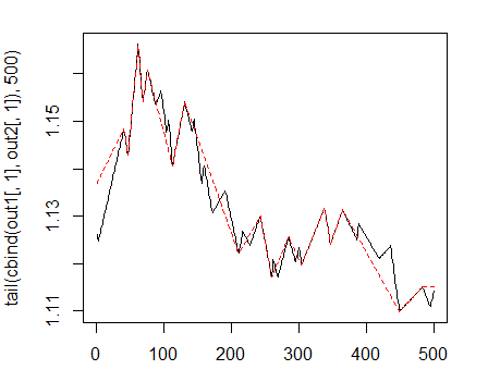
Fig. 1. Zigzags with minimum length of bends 25/75 p
Next we will use the first ZZ with a shorter leg. We are going to combine input variables and the target in the general dataframe, remove undefined data with a condition = "0" and remove the class "0" from the target.
> data <- cbind(as.data.frame(x) , Class = factor(out1[ ,2])) %>%
+               na.omit
> data <- data[data$Class != 0, ]
> data$Class <- rminer::delevels(data$Class, c("0", "1"), "1")
Look at the distribution of classes in the target:
> table(data$Class)

  -1    1
1980 1985
From what we can see, the classes are well balanced. Since we have a set of input and output data prepared, we can begin to evaluate the importance of predictors.
First we will check how correlated the input data is:
> descCor <- cor(data[ ,-ncol(data)])
> summary(descCor[upper.tri(descCor)])
    Min.  1st Qu.   Median     Mean  3rd Qu.     Max.
-0.20170  0.03803  0.26310  0.31750  0.57240  0.95730
Which input variables have correlation above 90%?
> highCor <- caret::findCorrelation(descCor, cutoff = .90)
> highCor
[1] 12 15
The answer is — rsi and SMI. We will form a set of data without these two and see the correlation of the remaining ones.
> data.f <- data[ ,-highCor]
> descCor <- cor(data.f[ ,-ncol(data.f)])
> summary(descCor[upper.tri(descCor)])
    Min.  1st Qu.   Median     Mean  3rd Qu.     Max.
-0.20170  0.03219  0.21610  0.27060  0.47820  0.89880
To evaluate the variable importance (VI) we will use a new package "Random Uniform Forests", which has a wide selection of instruments for its deep analysis and visualization. As per intent of the package's developers, the main objective of determining the importance of variables is to assess which, when, where and how they affect the problem being solved.
The package provides various importance measures of a variable in depth. We will consider them prior to going into deeper evaluation.
The Global Variable Importance sets variables that reduce the prediction error the utmost, but it doesn't tell us how the important variable affects the responses.
For example, we would like to know, which variables have a stronger influence over the separate class, or what is the interaction between variables.
The variable importance is measured by all units and trees, and that allows all variables to have a value, as the cutting points are accidental. Therefore, each variable has equal chances of being selected, but it will be getting the importance, only if it will be the one which mostly reduces the entropy in each node.
Local Variable Importance
Definition: A predictor is locally important in the first order, if for the same observation and all the trees it is the one with a highest frequency of occurrence in a terminal node.
Partial importance
Definition: A predictor is partially important, if for the same observation, class and on all orders it is the one that has the highest frequency of occurrence at the terminal node.
Interactions
We want to know, how predictors influence the problem, when we consider them. For example, some variables can have a relative low impact on the problem, but a strong impact on more relevant variables, or a variable can have a lot of interaction with others, which makes this variable influential. Let's define what interaction is.
Definition: A predictor interacts with another, if on the same observation and for all the trees both have, respectively, first and second highest frequency of occurrence in the terminal node.
Partial dependencies
These are the tools that allow to determine, how a variable (or a pair of variables) affects the value of response, knowing the values of all other variables. To be more specific, a partial dependence is the area where the maximum influence effect of the variable is exercised based on the value of response. The concept of a partial dependence arrived from Friedman (2002), who used it in Gradient Boosting Machines (GBM), however in Random Uniform Forests it was implemented differently.
In accordance with the ideas of the Random Uniform Forests package we can determine the importance of a variable based on the following scheme: Importance = contribution + interaction, where contribution is the influence of a variable (in respect to influencing all) on prediction errors, and interaction is an impact on other variables.
Let's proceed to experiments
We will divide our data set data.f[] into the training and testing sets with ratio 2/3, normalize in the range of -1;1 and test the model. For separation we will use the rminer::holdout() function which will divide the set in two. For normalization we use the caret::preProcess() function and the method = c("spatialSign"). When training the model the package will automatically parallelize calculations between available processor cores minus one using the "doParallel" package. You can indicate a specific number of cores to be used for calculation with the "threads" option.> idx <- rminer::holdout(y = data.f$Class)
> prep <- caret::preProcess(x = data.f[idx$tr, -ncol(data.f)],
+ method = c("spatialSign"))
> x.train <- predict(prep, data.f[idx$tr, -ncol(data.f)])
> x.test <- predict(prep, data.f[idx$ts, -ncol(data.f)])
> y.train <- data.f[idx$tr, ncol(data.f)]
> y.test <- data.f[idx$ts, ncol(data.f)]
> ruf <- randomUniformForest( X = x.train,
+ Y = y.train,
+ xtest = x.test,
+ ytest = y.test,
+ mtry = 1, ntree = 300,
+ threads = 2,
+ nodesize = 2
+ )
Labels -1 1 have been converted to 1 2 for ease of computation and will be used internally as a replacement.
> print(ruf)
Call:
randomUniformForest.default(X = x.train, Y = y.train, xtest = x.test,
ytest = y.test, ntree = 300, mtry = 1, nodesize = 2, threads = 2)
Type of random uniform forest: Classification
paramsObject
ntree 300
mtry 1
nodesize 2
maxnodes Inf
replace TRUE
bagging FALSE
depth Inf
depthcontrol FALSE
OOB TRUE
importance TRUE
subsamplerate 1
classwt FALSE
classcutoff FALSE
oversampling FALSE
outputperturbationsampling FALSE
targetclass -1
rebalancedsampling FALSE
randomcombination FALSE
randomfeature FALSE
categorical variables FALSE
featureselectionrule entropy
Out-of-bag (OOB) evaluation
OOB estimate of error rate: 20.2%
OOB error rate bound (with 1% deviation): 21.26%
OOB confusion matrix:
Reference
Prediction -1 1 class.error
-1 1066 280 0.2080
1 254 1043 0.1958
OOB estimate of AUC: 0.798
OOB estimate of AUPR: 0.7191
OOB estimate of F1-score: 0.7962
OOB (adjusted) estimate of geometric mean: 0.7979
Breiman's bounds
Expected prediction error (under approximatively balanced classes): 18.42%
Upper bound: 27.76%
Average correlation between trees: 0.0472
Strength (margin): 0.4516
Standard deviation of strength: 0.2379
Test set
Error rate: 19.97%
Confusion matrix:
Reference
Prediction -1 1 class.error
-1 541 145 0.2114
1 119 517 0.1871
Area Under ROC Curve: 0.8003
Area Under Precision-Recall Curve: 0.7994
F1 score: 0.7966
Geometric mean: 0.8001
We will decipher this slightly:
- Training error (internal error) given 1% of a deviation = 21.26%.
- Breiman's bounds — theoretical properties proposed by Breiman (2001). Since the Random Uniform Forests inherits the properties of Random Forests, they are applicable here. For classification it gives two borders of prediction error, average correlation between trees, strength and standard deviation of strength.
- Expected prediction error = 18.42%. The upper limit error = 27.76%.
- Testing error = 19.97% (external error). (If the external evaluation is less or equals the internal evaluation and less than the upper limit of Breiman's bounds, then a retraining most probably won't occur.)
Let's see the chart of a training error:
> plot(ruf)
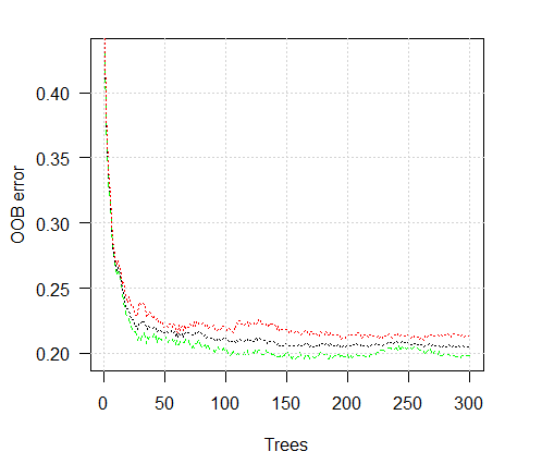
Fig. 2. Training error depending on the number of trees
> summary(ruf)

Global Variable importance:
Note: most predictive features are ordered by 'score' and plotted.
Most discriminant ones should also be taken into account by looking 'class'
and 'class.frequency'.

   variables score class class.frequency percent
1        cci  2568     1            0.50  100.00
2     signal  2438     1            0.51   94.92
3      slowD  2437     1            0.51   94.90
4       oscK  2410     1            0.50   93.85
5        ADX  2400    -1            0.51   93.44
6        vol  2395     1            0.51   93.24
7        atr  2392    -1            0.51   93.15
8       sign  2388     1            0.50   92.97
9       vsig  2383     1            0.50   92.81
10        ar  2363    -1            0.51   92.01
11       chv  2327    -1            0.50   90.62
12       cmo  2318    -1            0.51   90.28
13        DX  2314     1            0.50   90.10
14     oscDX  2302    -1            0.51   89.64
15        tr  2217     1            0.52   86.31
   percent.importance
1                   7
2                   7
3                   7
4                   7
5                   7
6                   7
7                   7
8                   7
9                   7
10                  7
11                  7
12                  7
13                  6
14                  6
15                  6

Average tree size (number of nodes) summary:
   Min. 1st Qu.  Median    Mean 3rd Qu.    Max.
      3    1044    1313    1213    1524    1861

Average Leaf nodes (number of terminal nodes) summary:
   Min. 1st Qu.  Median    Mean 3rd Qu.    Max.
      2     522     657     607     762     931

Leaf nodes size (number of observations per leaf node) summary:
    Min.  1st Qu.   Median     Mean  3rd Qu.     Max.
   1.000    1.000    2.000    4.355    3.000 2632.000

Average tree depth : 10

Theoretical (balanced) tree depth : 11
We see that all our input variables are significant and important. It is indicated, in which classes the variables appear most frequently.
And some more statistics:
> pr.ruf <- predict(ruf, x.test, type = "response");
> ms.ruf <- model.stats(pr.ruf, y.test)
Test set
Error rate: 19.97%

Confusion matrix:
          Reference
Prediction  -1   1 class.error
        -1 540 144      0.2105
        1  120 518      0.1881

Area Under ROC Curve: 0.8003
Area Under Precision-Recall Curve: 0.7991
F1-score: 0.7969
Geometric mean: 0.8001
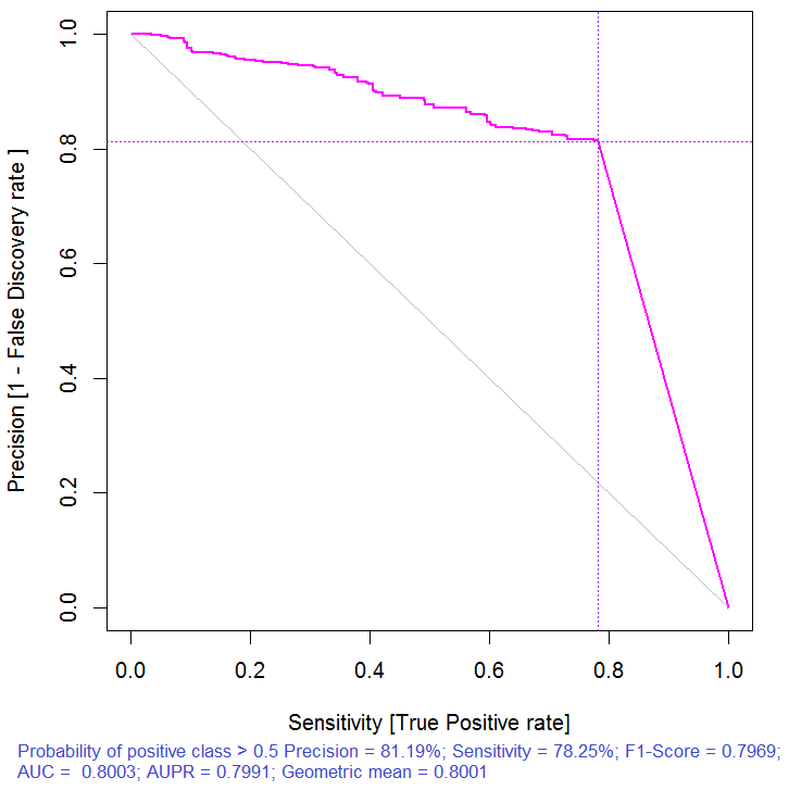
Fig. 3. Precision-recall curve
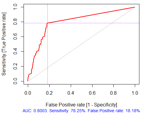
Fig. 4. ROC curve or error curve
If we stop right here, which is normally offered by many filter packages, we would have to select several predictors with the best indicators of global importance. This choice does not provide good results as it does not take into account the mutual influence of the predictors.
> imp.ruf <- importance(ruf, Xtest = x.test, maxInteractions = 3)

1 - Global Variable Importance (15 most important based on information gain) :
Note: most predictive features are ordered by 'score' and plotted.
Most discriminant ones should also be taken into account by looking 'class'
and 'class.frequency'.

   variables score class class.frequency percent
1        cci  2568     1            0.50  100.00
2     signal  2438     1            0.51   94.92
3      slowD  2437     1            0.51   94.90
4       oscK  2410     1            0.50   93.85
5        ADX  2400    -1            0.51   93.44
6        vol  2395     1            0.51   93.24
7        atr  2392    -1            0.51   93.15
8       sign  2388     1            0.50   92.97
9       vsig  2383     1            0.50   92.81
10        ar  2363    -1            0.51   92.01
11       chv  2327    -1            0.50   90.62
12       cmo  2318    -1            0.51   90.28
13        DX  2314     1            0.50   90.10
14     oscDX  2302    -1            0.51   89.64
15        tr  2217     1            0.52   86.31
   percent.importance
1                   7
2                   7
3                   7
4                   7
5                   7
6                   7
7                   7
8                   7
9                   7
10                  7
11                  7
12                  7
13                  6
14                  6
15                  6


2 - Local Variable importance
Variables interactions (10 most important variables at first (columns) and second (rows) order) :
For each variable (at each order), its interaction with others is computed.

                cci    cmo  slowD   oscK signal    atr    chv
cmo          0.1933 0.1893 0.1345 0.1261 0.1146 0.1088 0.1062
cci          0.1770 0.1730 0.1182 0.1098 0.0983 0.0925 0.0899
slowD        0.1615 0.1575 0.1027 0.0943 0.0828 0.0770 0.0744
signal       0.1570 0.1530 0.0981 0.0897 0.0782 0.0725 0.0698
atr          0.1490 0.1450 0.0902 0.0818 0.0703 0.0646 0.0619
ADX          0.1468 0.1428 0.0879 0.0795 0.0680 0.0623 0.0596
ar           0.1452 0.1413 0.0864 0.0780 0.0665 0.0608 0.0581
oscK         0.1441 0.1401 0.0853 0.0769 0.0654 0.0596 0.0570
DX           0.1407 0.1367 0.0819 0.0735 0.0620 0.0562 0.0536
oscDX        0.1396 0.1356 0.0807 0.0723 0.0608 0.0551 0.0524
avg1rstOrder 0.1483 0.1443 0.0895 0.0811 0.0696 0.0638 0.0612
                ADX     tr     ar   vsig     DX  oscDX   sign
cmo          0.1026 0.1022 0.1013 0.1000 0.0977 0.0973 0.0964
cci          0.0864 0.0859 0.0850 0.0837 0.0815 0.0810 0.0802
slowD        0.0708 0.0704 0.0695 0.0682 0.0660 0.0655 0.0647
signal       0.0663 0.0659 0.0650 0.0637 0.0614 0.0610 0.0601
atr          0.0584 0.0579 0.0570 0.0557 0.0535 0.0531 0.0522
ADX          0.0561 0.0557 0.0548 0.0534 0.0512 0.0508 0.0499
ar           0.0546 0.0541 0.0533 0.0519 0.0497 0.0493 0.0484
oscK         0.0534 0.0530 0.0521 0.0508 0.0486 0.0481 0.0473
DX           0.0500 0.0496 0.0487 0.0474 0.0452 0.0447 0.0439
oscDX        0.0489 0.0485 0.0476 0.0463 0.0440 0.0436 0.0427
avg1rstOrder 0.0577 0.0572 0.0563 0.0550 0.0528 0.0524 0.0515
                vol avg2ndOrder
cmo          0.0889      0.1173
cci          0.0726      0.1010
slowD        0.0571      0.0855
signal       0.0526      0.0810
atr          0.0447      0.0730
ADX          0.0424      0.0707
ar           0.0409      0.0692
oscK         0.0397      0.0681
DX           0.0363      0.0647
oscDX        0.0352      0.0636
avg1rstOrder 0.0439      0.0000


Variable Importance based on interactions (10 most important) :
   cmo    cci  slowD signal   oscK    atr    ADX     ar
0.1447 0.1419 0.0877 0.0716 0.0674 0.0621 0.0563 0.0533
   chv     DX
0.0520 0.0485

Variable importance over labels (10 most important variables
conditionally to each label) :
       Class -1 Class 1
cci        0.16    0.23
cmo        0.20    0.18
slowD      0.09    0.10
oscK       0.09    0.07
signal     0.05    0.07
tr         0.02    0.07
ADX        0.06    0.03
chv        0.06    0.04
atr        0.05    0.06
ar         0.05    0.03
From what we see, the importance of variables on the basis of interaction with others highlights the top 10 that don't match the order of global importance. And finally, the importance of variables by classes taking into account their contribution and involvement. Please note that the variable tr, which on the basis of global importance was at the last place and, in theory, should have been abandoned, has actually risen to the sixth place due to the strong interaction.
Thus, top 10 variables:
> best <- Cs(cci, cmo, slowD, oscK, signal, tr, ADX. chv, atr, ar)Let's check, how the model's quality has improved with the set of most important predictors.
> x.tr <- x.train[ ,best]
> x.tst <- x.test[ ,best]
> ruf.opt <- randomUniformForest(X = x.tr,
+                                Y = y.train,
+                                xtest = x.tst,
+                                ytest = y.test,
+                                ntree = 300,
+                                mtry = "random",
+                                nodesize = 1,
+                                threads = 2)
Labels -1 1 have been converted to 1 2 for ease of computation
and will be used internally as a replacement.
> ruf.opt
Call:
randomUniformForest.default(X = x.tr, Y = y.train, xtest = x.tst,
    ytest = y.test, ntree = 300, mtry = "random", nodesize = 1,
    threads = 2)

Type of random uniform forest: Classification

                           paramsObject
ntree                               300
mtry                             random
nodesize                              1
maxnodes                            Inf
replace                            TRUE
bagging                           FALSE
depth                               Inf
depthcontrol                      FALSE
OOB                                TRUE
importance                         TRUE
subsamplerate                         1
classwt                           FALSE
classcutoff                       FALSE
oversampling                      FALSE
outputperturbationsampling        FALSE
targetclass                          -1
rebalancedsampling                FALSE
randomcombination                 FALSE
randomfeature                     FALSE
categorical variables             FALSE
featureselectionrule            entropy

Out-of-bag (OOB) evaluation
OOB estimate of error rate: 18.69%
OOB error rate bound (with 1% deviation): 19.67%

OOB confusion matrix:
          Reference
Prediction   -1    1 class.error
        -1 1079  253      0.1899
        1   241 1070      0.1838

OOB estimate of AUC: 0.8131
OOB estimate of AUPR: 0.7381
OOB estimate of F1-score: 0.8125
OOB (adjusted) estimate of geometric mean: 0.8131

Breiman's bounds
Expected prediction error (under approximatively balanced classes): 14.98%
Upper bound: 28.18%
Average correlation between trees: 0.0666
Strength (margin): 0.5548
Standard deviation of strength: 0.2945

> pr.ruf.opt <- predict(ruf.opt, x.tst, type = "response")
> ms.ruf.opt <- model.stats(pr.ruf.opt, y.test)
Test set
Error rate: 17.55%

Confusion matrix:
          Reference
Prediction  -1   1 class.error
        -1 552 124      0.1834
        1  108 538      0.1672
Area Under ROC Curve: 0.8245
Area Under Precision-Recall Curve: 0.8212
F1-score: 0.8226
Geometric mean: 0.8244
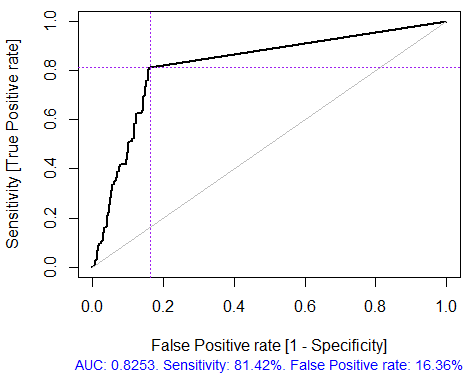
Fig. 5. ROC curve or error curve
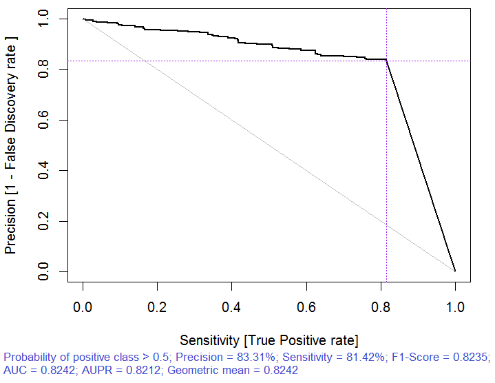
Fig. 6. Precision-recall curve
The quality has clearly improved. The prediction error on the test set 17.55% is lower than the upper level 28.18%, therefore retraining is highly unlikely. The model has many other hyperparameters, whose tuning may allow further enhancement of the model's quality, however, this is not the current article's goal.
> imp.ruf.opt <- importance(ruf.opt, Xtest = x.tst)

 Relevant variables have been extracted.

1 - Global Variable Importance (10 most important based on information gain) :
Note: most predictive features are ordered by 'score' and plotted.
Most discriminant ones should also be taken into account by looking 'class'
and 'class.frequency'.

   variables score class class.frequency percent
1        atr  3556    -1            0.50  100.00
2       oscK  3487    -1            0.51   98.07
3        chv  3465     1            0.51   97.45
4     signal  3432     1            0.51   96.51
5        cci  3424     1            0.50   96.30
6      slowD  3415     1            0.51   96.04
7        ADX  3397    -1            0.50   95.52
8         ar  3369    -1            0.50   94.76
9         tr  3221     1            0.53   90.59
10       cmo  3177    -1            0.50   89.36
   percent.importance
1                  10
2                  10
3                  10
4                  10
5                  10
6                  10
7                  10
8                  10
9                   9
10                  9


2 - Local Variable importance
Variables interactions (10 most important variables at first (columns) and second (rows) order) :
For each variable (at each order), its interaction with others is computed.

                atr    cci   oscK  slowD    ADX     tr    chv
cci          0.1748 0.1625 0.1620 0.1439 0.1411 0.1373 0.1349
atr          0.1650 0.1526 0.1522 0.1341 0.1312 0.1274 0.1251
oscK         0.1586 0.1462 0.1457 0.1277 0.1248 0.1210 0.1186
chv          0.1499 0.1375 0.1370 0.1190 0.1161 0.1123 0.1099
ar           0.1450 0.1326 0.1321 0.1140 0.1112 0.1074 0.1050
signal       0.1423 0.1300 0.1295 0.1114 0.1085 0.1047 0.1024
ADX          0.1397 0.1273 0.1268 0.1088 0.1059 0.1021 0.0997
slowD        0.1385 0.1262 0.1257 0.1076 0.1048 0.1010 0.0986
cmo          0.1276 0.1152 0.1147 0.0967 0.0938 0.0900 0.0876
tr           0.1242 0.1118 0.1113 0.0932 0.0904 0.0866 0.0842
avg1rstOrder 0.1466 0.1342 0.1337 0.1156 0.1128 0.1090 0.1066
             signal     ar    cmo avg2ndOrder
cci          0.1282 0.1182 0.1087      0.1412
atr          0.1184 0.1084 0.0989      0.1313
oscK         0.1120 0.1020 0.0925      0.1249
chv          0.1033 0.0933 0.0838      0.1162
ar           0.0984 0.0884 0.0789      0.1113
signal       0.0957 0.0857 0.0762      0.1086
ADX          0.0931 0.0831 0.0736      0.1060
slowD        0.0919 0.0819 0.0724      0.1049
cmo          0.0810 0.0710 0.0615      0.0939
tr           0.0776 0.0676 0.0581      0.0905
avg1rstOrder 0.0999 0.0900 0.0804      0.0000


Variable Importance based on interactions (10 most important) :
   atr    cci   oscK    chv  slowD    ADX signal     ar
0.1341 0.1335 0.1218 0.0978 0.0955 0.0952 0.0898 0.0849
    tr    cmo
0.0802 0.0672

Variable importance over labels
(10 most important variables conditionally to each label) :
       Class -1 Class 1
atr        0.17    0.14
oscK       0.16    0.11
tr         0.03    0.16
cci        0.14    0.13
slowD      0.12    0.09
ADX        0.10    0.10
chv        0.08    0.10
signal     0.09    0.07
cmo        0.07    0.03
ar         0.06    0.06
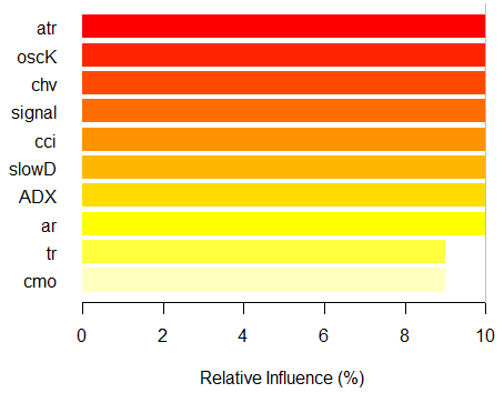
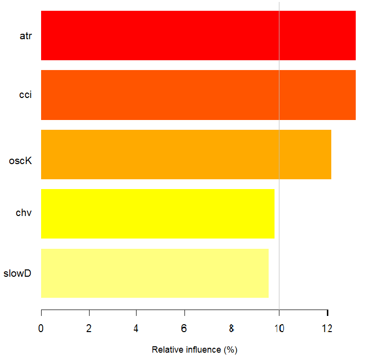
Fig. 7. The importance of variables based on the information gain
As we can see, the global importance of variables has almost leveled off, but the importance of variables by classes is ranked differently. The tr variable takes the third place.
Partial dependence over predictor
The partial dependence of the most important variables will be considered.
> plot(imp.ruf.opt, Xtest = x.tst)
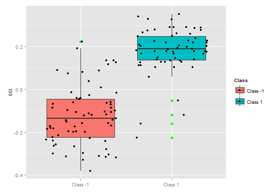
Fig. 8. Partial dependence of cci variable
> pd.signal <- partialDependenceOverResponses(x.tst,
+                                            imp.ruf.opt,
+                                            whichFeature = "signal",
+                                            whichOrder = "all"
+ )
Fig. 9. Partial dependence of the signal variable
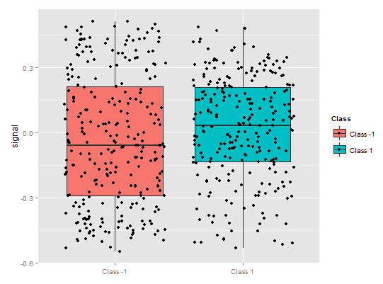
There is quite a different picture of a partial dependence for the signal predicator in the figure above. Almost complete data coverage for both classes is observed.
> pd.tr <- partialDependenceOverResponses(x.tst,
                                          imp.ruf.opt,
                                          whichFeature = "tr",
                                          whichOrder = "all"
                                          )
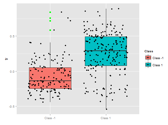
A partial dependency of the tr predicator shows reasonable separation by classes, still there is a considerable coverage here.
Fig. 10. Partial dependence of tr variable
> pd.chv <- partialDependenceOverResponses(x.tst,
                                           imp.ruf.opt,
                                           whichFeature = "chv",
                                           whichOrder = "all")
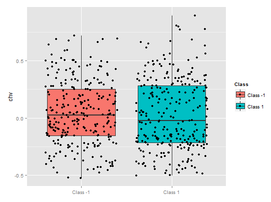
A partial dependence of the chv predicator is absolutely deplorable. A complete data coverage by classes is observed.
Fig. 11. Partial dependence of the chv variable
This way we can visually determine, how the predictor data is linked to the classes, and how separable they are.
The importance of variable over classes
"The importance of variable" over classes provides a local perspective: the class is fixed, which means that first is the decision to fix the class considering the variables which are important and act as constants, and, eventually, the important variables for each class are considered. Hence, every variable has importance, as if there were no other classes.
Here we are not interested in variables that led to choosing a class, but variables which will be important in the class, when the latter will be selected. The order of variables gives their free ranking regarding their rank in each class without consideration of class importance.
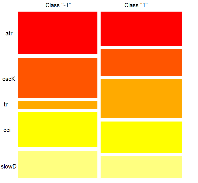
What does the chart show? The tr predictor is considerably more important for the "1" class than for the "-1" class. And vice versa, the predictor oscK for the class "-1" is more important than for the "1" class. Predictors have different importance in different classes.
Fig. 12. Importance of variables by classes
The importance of variables based on interaction
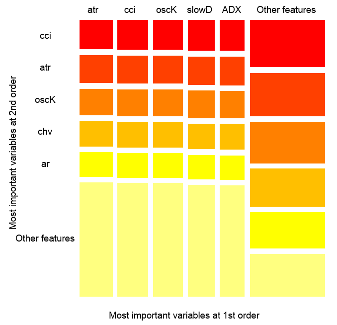
The chart below shows, how each variable is presented in the joint interaction with any other variable. One important remark: the first variable is not necessarily the most important, instead, it is the one that has the greatest mutual impact with others.Variables interactions over observations
Fig. 14. The importance of variables over observations
The figure above shows the interaction of the first and second order for all predictors in accordance with the definition, that we gave for interaction. Its area equals unity. The first order indicates that variables (sorted by descending influence) are most important, if the decision has to be made taking into account only one variable. The second order indicates, that if the unknown variable is already selected in the first order, then the second most important variable will be one of those in the second order.
For clarification, the interaction provides a table of ordered features. The first order gives ordered opportunities of most important variables. The second order gives ordered opportunities of second most important variables. The intersection of a pair of variables gives their relative mutual influence out of all possible mutual influences. Please note that these measurements depend on both model and data. Therefore, the confidence in measurements directly depends on the confidence in predictions. We can also add, that a meta-variable called "other signs" occurs, which means that we allow the algorithm to show the default view for the visualization of the less relevant grouped variables.
Partial importance
You can look at the partial importance based on x.tst observations over the class "-1".
> par.imp.ruf <- partialImportance(X = x.tst,
+                                  imp.ruf.opt,
+                                  whichClass = "-1")
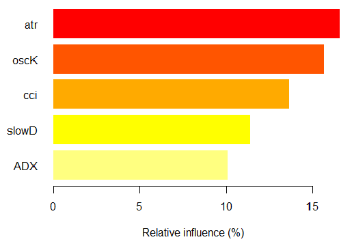
Relative influence: 67.41%
Based on x.tst  and class «-1»
Fig. 15. Partial importance of variables based on observations over the class "-1"
As we see, the most important predictors of the class "-1" are five predictors shown on the figure above.
Now the same for the class "+1"
> par.imp.ruf <- partialImportance(X = x.tst,
+                                  imp.ruf.opt,
+                                  whichClass = "1")
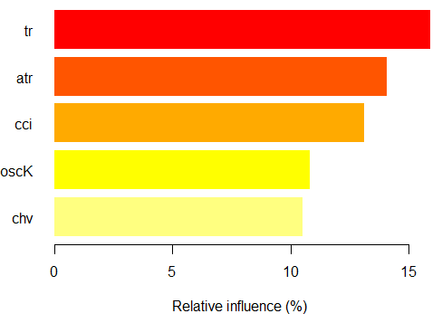
Relative influence: 64.45%
Fig. 16. Partial importance of variables based on observations over the class "+1"
We see, that the predictors are different both in structure and rankings.
Let's see the partial dependency between predictors cci and atr, that are the most important in the first and the second order of predictor interaction.
> par.dep.1 <- partialDependenceBetweenPredictors(Xtest = x.tst,
+                             imp.ruf.opt,
+                             features = Cs(atr, cci),
+                             whichOrder = "all",
+                             perspective = T)

Level of interactions between atr and cci at first order: 0.1748
(99.97% of the feature(s) with maximum level)
Level of interactions between atr and cci at second order: 0.1526
(87.28% of the feature(s) with maximum level)

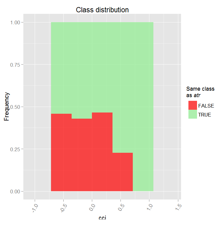
Class distribution : for a variable of the pair, displays the estimated
probability that the considered variable has the same class than the other.
If same class tends to be TRUE then the variable has possibly an influence
on the other (for the considered category or values)when predicting a label.

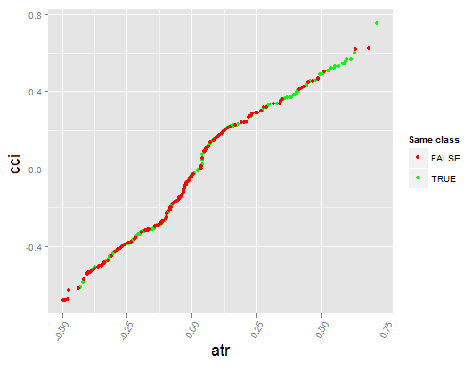
Dependence : for the pair of variables, displays the shape of their
dependence and the estimated agreement in predicting the same class,
for the values that define dependence. In case of categorical variables,
cross-tabulation is used.

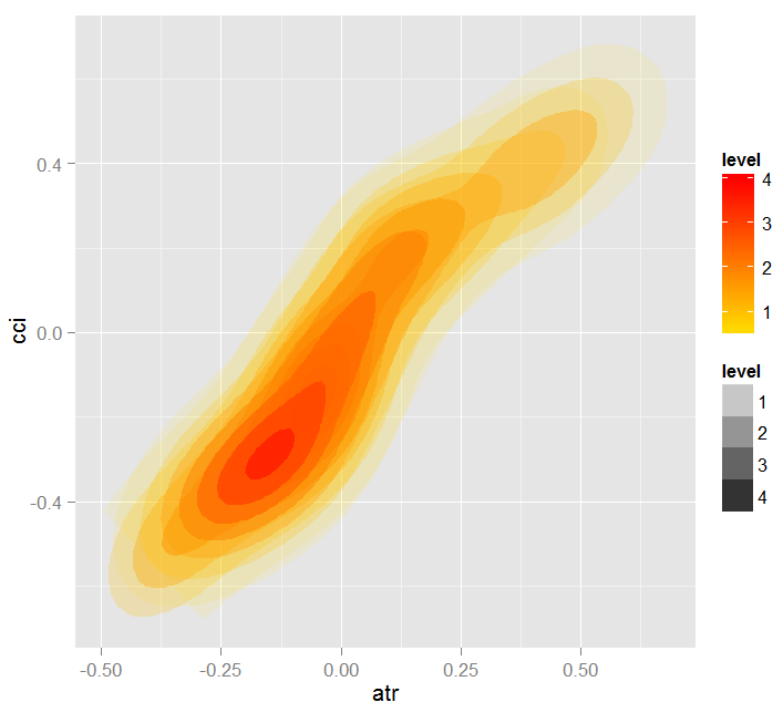
Heatmap : for the pair of variables, displays the area where the dependence
is the most effective.
The darker the colour, the stronger is the dependence.

From the pair of variables, the one that dominates is, possibly, the one
that is the most discriminant one (looking 'Global variable Importance')
and/or the one that has the higher level of interactions(looking
'Variable Importance based on interactions').
Fig. 17. Partial dependency between predictors cci and atr
Fig. 18. Dependence between predictors atr and cci
Fig. 19. Heatmap of dependence between predictors atr and cci
Global variable importance was determined to describe which global variables have the greatest influence on reducing the prediction errors.
Local variable importance describes what makes a variable influential by using its interaction with others.
This leads to partial importance which shows when a variable is more important. The last step in analyzing the importance of variable is a partial dependence that sets when and/or how each variable is associated with a response.
To summarize: a variable importance in the Random Uniform Forests goes from the highest to the lowest level with detailing. Firstly, we find out which variables are important, and learn weight nuances in each class. Then we find out what makes them influential considering their interaction and choose a variable first considering all classes as one. The next step — we learn where they obtain their influence considering within each class when it is fixed. Finally, we obtain when and how the variable can be/is important by looking at the "partial dependency". All measurements, except for "global variable of importance", operate on any training or testing set.
A presented multilevel assessment of predictors allows to select the most important predictors and create optimal sets by significantly reducing data dimension and improving the quality of predictions.
You can evaluate and choose not only predictors but also the most informative observation items.
Let's look at the another interesting package — "RoughSet".
Brief description: There are two main sections covered in this package: the Rough Set Theory (RST) and the Fuzzy Rough Set Theory (FRST)). RST was proposed by Z. Pawlak (1982, 1991), it provides sophisticated mathematical instruments for modeling and analyzing information systems which include the heterogeneity and inaccuracies. Using the indistinguishability relationships between objects RST does not require additional parameters to extract information.
The FRST theory, RST extension, was proposed by D. Dubois and H. Prade (1990), it combines the concepts of uncertainty and indistinguishability which are expressed in fuzzy sets proposed by L.A. Zadeh (1965) and RST. This concept allows you to analyze continuous attributes (variables) without preliminary data discretization. Based on the above-described concepts many methods have been proposed and used in several different areas. In order to solve problems the methods use the relation of indistinguishability and the concept of lower and upper approximation.
Please allow me a small digression.
A method of knowledge representation usually plays a major role in the information system. The best-known methods of presenting knowledge in the systems of inductive concept formation are: production rules, decision trees, predicate calculation and semantic networks.
For extracting and generalizing knowledge stored in the actual informational arrays the following main problems appear:
- This data is dissimilar (quantitative, qualitative, structural).
- Actual databases are normally large, therefore exponential complexity algorithms for retrieving knowledge from the database may appear unacceptable.
- The information contained in the actual data arrays can be incomplete, excessive, distorted, controversial, and some values of a number of attributes may be completely absent. Therefore, for construction of classification rules you should use only the existing attributes.
Currently for extracting knowledge from the database (Data Mining) the rough sets theory is being increasingly used as a theoretical framework and a set of practical methods.
Approximate sets have undefined boundaries, i.e. they can't be accurately described by a set of features available.
A theory of approximate sets was proposed by Zdzislaw Pawlak in 1982 and became a new mathematical instrument for operation with incomplete information. The most important concept of this theory is a so-called upper and lower approximation of the approximate sets that allows to assess the possibility or the necessity of the element's belonging to a set with "fuzzy" boundaries.
The lower approximation consists of elements that definitely belong to X, higher approximation contains elements that possibly belong to X. The boundary region of the X set is the difference between higher and lower approximation, i.e. the boundary region has elements of the X set that belong to a higher approximation other than a lower approximation.
A simple but powerful concept of approximate sets became a base for multiple theoretical studies — logic, algebra, topology and applied studies — artificial intelligence, approximate reasoning, intellectual data analysis, decision theory, image processing and pattern recognition.
The concept of "approximate set" deals with "data imperfection" related to "granularity" of information. This concept is inherently topological and complements other well-known approaches used for operation with incomplete information, such as fuzzy sets, Bayesian reasoning, neural networks, evolutionary algorithms, statistical methods of data analysis.
Let's proceed. All methods provided in this package can be grouped accordingly:
Basic concepts of RST and FRST. In this part we can observe four different tasks: indiscernibility relation, lower and upper approximation, positive region and discernibility matrix.
Discretization. It is used to convert physical data into nominal. From the RST perspective this task tries to maintain the discernibility between objects.
Feature selection. This is a process of finding subsets of predictors that are trying to obtain the same quality as the full set of predictors. In other words, the aim is to select the essential features and to eliminate their dependence. It is useful and necessary when we are faced with a set of data containing multiple features. In terms of RST and FRST the choice of predictors relates to the search of superreducts and reducts.
Instance selection. This process is aimed at removing noisy, unnecessary or conflicting copies from the training data set while saving the coherent. Thus, a good classification accuracy is achieved by removing the specimens that do not give a positive contribution.
Rule induction. As we have already mentioned, the task of inducing rules is used for generating rules, providing knowledge of the solution table. Typically, this process is called a training phase in the machine learning.
Prediction/classification. This task is used to predict values of a variable from the new data set (test set).
We will explore only two categories from this list — choice of predictors and selection of samples.
Let's form the set of input and output data. We will use the same data that we have obtained before, but will transform it into the "DecisionTable" class that the package operates with.> library(RoughSets) Loading required package: Rcpp > require(magrittr) > data.tr <- SF.asDecisionTable(data.f[idx$tr, ], + decision.attr = 16, + indx.nominal = 16) > data.tst <- SF.asDecisionTable(data.f[idx$ts, ], + decision.attr = 16, + indx.nominal = 16 + ) > true.class <- data.tst[ ,ncol(data.tst)]As we have previously mentioned, RST uses nominal data. Since we have continuous numerical data we are going to convert it into nominal data using a specialized discretization function available from the package.
> cut.values <- D.global.discernibility.heuristic.RST(data.tr)
> data.tr.d <- SF.applyDecTable(data.tr, cut.values)
Let's see what we obtain as a result:
> summary(data.tr.d)
           DX                ADX
 (12.5,20.7]: 588   (17.6,19.4]: 300
 (20.7, Inf]:1106   (19.4,25.4]: 601
 [-Inf,12.5]: 948   (25.4,31.9]: 294
                    (31.9, Inf]: 343
                    [-Inf,17.6]:1104

         oscDX                 ar
 (1.81, Inf]:1502   (-40.6,40.6]:999
 [-Inf,1.81]:1140   (40.6,71.9] :453
                    (71.9, Inf] :377
                    [-Inf,-40.6]:813


                   tr                     atr
 (0.000205,0.000365]:395   (0.00072,0.00123]:1077
 (0.000365,0.0005]  :292   (0.00123, Inf]   : 277
 (0.0005,0.00102]   :733   [-Inf,0.00072]   :1288
 (0.00102,0.00196]  :489
 (0.00196, Inf]     :203
 [-Inf,0.000205]    :530
           cci                   chv
 (-6.61, Inf]:1356   (-0.398,0.185]:1080
 [-Inf,-6.61]:1286   (0.185,0.588] : 544
                     (0.588, Inf]  : 511
                     [-Inf,-0.398] : 507


          cmo                sign
 (5.81,54.1]: 930   [-Inf, Inf]:2642
 (54.1, Inf]: 232
 [-Inf,5.81]:1480


            vsig              slowD
 (0.0252, Inf]:1005   [-Inf, Inf]:2642
 [-Inf,0.0252]:1637


                 oscK              signal
 (-0.0403,0.000545]:633   (-11.4, Inf]:1499
 (0.000545,0.033]  :493   [-Inf,-11.4]:1143
 (0.033, Inf]      :824
 [-Inf,-0.0403]    :692


               vol      Class
 (0.0055,0.00779]:394   -1:1319
 (0.00779,0.0112]:756   1 :1323
 (0.0112,0.0154] :671
 (0.0154, Inf]   :670
 [-Inf,0.0055]   :151
We see that the predictors are discretized differently. Variables like slowD, sign are not separated at all. Variables signal, vsig, cci, oscDX are simply divided into two areas. The other variables are divided between 3 and 6 classes.
We will select the important variables:
> reduct1 <- FS.quickreduct.RST(data.tr.d, control = list())
> best1 <- reduct1$reduct
> best1
    DX    ADX  oscDX     ar     tr    atr    cci
     1      2      3      4      5      6      7
   chv    cmo   vsig   oscK signal    vol
     8      9     11     13     14     15
Data that wasn't divided (slowD, sign) is removed from the set. We will carry out the test set discretization and transform it according to the reduction carried out.
> data.tst.d <- SF.applyDecTable(data.tst, cut.values)
> new.data.tr <- SF.applyDecTable(data.tr.d, reduct1)
> new.data.tst <- SF.applyDecTable(data.tst.d, reduct1)
Now, using one excellent opportunity of the package called "induction rules" we will extract a set of rules that bind predictors and a target. One of the following options will be used:
> rules <- RI.AQRules.RST(new.data.tr, confidence = 0.9, timesCovered = 3)
We will check on the test set, how these rules work at predicting:
> pred.vals <- predict(rules, new.data.tst)
> table(pred.vals)
pred.vals
 -1   1
655 667
Metrics:
> caret::confusionMatrix(true.class, pred.vals[ ,1])
Confusion Matrix and Statistics

          Reference
Prediction  -1   1
        -1 497 163
        1  158 504

               Accuracy : 0.7572
                 95% CI : (0.7331, 0.7801)
    No Information Rate : 0.5045
    P-Value [Acc > NIR] : <2e-16

                  Kappa : 0.5144
 Mcnemar's Test P-Value : 0.8233

            Sensitivity : 0.7588
            Specificity : 0.7556
         Pos Pred Value : 0.7530
         Neg Pred Value : 0.7613
             Prevalence : 0.4955
         Detection Rate : 0.3759
   Detection Prevalence : 0.4992
      Balanced Accuracy : 0.7572

       'Positive' Class : -1
And now — a choice of significant examples:
> ##-----Instance Selection-----------
> res.1 <- IS.FRIS.FRST(decision.table = data.tr,
                        control = list(threshold.tau = 0.5, alpha = 1,
                        type.aggregation = c("t.tnorm", "lukasiewicz"),
                        t.implicator = "lukasiewicz"))
> new.data.tr <- SF.applyDecTable(data.tr, res.1)

> nrow(new.data.tr)
[1] 2353
Approximately 300 examples were rated as minor and discarded. We will extract a set of rules from this set and compare the quality of prediction with a previous set.
> rules <- RI.AQRules.RST(new.data.tr, confidence = 0.9,
                          timesCovered = 3)
> pred.vals <- predict(rules, new.data.tst)
> table(pred.vals)
pred.vals
 -1   1
638 684
> caret::confusionMatrix(true.class, pred.vals[ ,1])
Confusion Matrix and Statistics

          Reference
Prediction  -1   1
        -1 506 154
        1  132 530

               Accuracy : 0.7837
                 95% CI : (0.7605, 0.8056)
    No Information Rate : 0.5174
    P-Value [Acc > NIR] : <2e-16

                  Kappa : 0.5673
 Mcnemar's Test P-Value : 0.2143

            Sensitivity : 0.7931
            Specificity : 0.7749
         Pos Pred Value : 0.7667
         Neg Pred Value : 0.8006
             Prevalence : 0.4826
         Detection Rate : 0.3828
   Detection Prevalence : 0.4992
      Balanced Accuracy : 0.7840

       'Positive' Class : -1
The quality is higher than in the previous case. It should be noted that, as in the case with RandomUniformForests, it is impossible to obtain reproducible results in the repeated experiments. Each new launch gives a slightly different result.
How do the rules look? Let's see:> head(rules) [[1]] [[1]]$idx [1] 6 4 11 [[1]]$values [1] "(85.1, Inf]" "(0.00137, Inf]" "(0.0374, Inf]" [[1]]$consequent [1] "1" [[1]]$support [1] 1335 1349 1363 1368 1372 1390 1407 1424 1449 1454 [11] 1461 1472 1533 1546 1588 1590 1600 1625 1630 1661 [21] 1667 1704 1720 1742 1771 1777 1816 1835 1851 1877 [31] 1883 1903 1907 1912 1913 1920 1933 1946 1955 1981 [41] 1982 1998 2002 2039 2040 2099 2107 2126 2128 2191 [51] 2195 2254 2272 2298 2301 2326 2355 2356 2369 2396 [61] 2472 2489 2497 2531 2564 2583 2602 2643 [[1]]$laplace 1 0.9857143
This is a list containing the following data:
- $idx — index predictors participating in this rule. In the example above these are 6("atr") , 4("ar") and 11("vsig").
- $values — a range of value indicators where this rule operates.
- $consequent — solution: class = "1". To make it sound understandable: if "atr" is in the range "(85.1, Inf]" AND "ar" is in the range "(0.00137, Inf]" AND "vsig" is in the range "(0.0374, Inf]", THEN Class = "1".
- $support — indexes of examples supporting this solution.
- $laplace — an assessment of confidence level for this rule.
A calculation of rules takes considerable time.
Conclusion
We have considered new opportunities based on predictor assessment, their visualization and choosing the most valuable. We also have examined different levels of importance, predictor dependencies and their impact on responses. The results of experiments will be applied in the next article, where we will consider deep networks with RBM.
Translated from Russian by MetaQuotes Ltd.
Original article: https://www.mql5.com/ru/articles/2029
 Error Handling and Logging in MQL5
 Indicator for Spindles Charting
- Free trading apps
- Over 8,000 signals for copying
- Economic news for exploring financial markets
You agree to website policy and terms of use
Read this post can be useful:
Can Math Beat Financial Markets?
https://www.mql5.com/en/users/mgsystem/blog
Hi Vladimir,
Forgive me this silly question but I'm currently trying to construct my own ( very simple ) model starting from your nice example and I'm wondering why you're shifting the ZZ's differences forward in the ZZ function :
...I mean, after all, we want to train a model to predict the FUTURE value of the Zigzag, so what's the point in training a model using predictors ( technical indicators ) that summarize the market quotes at the end of day N with a target value which is the sign of the difference between the Zigzag value of day N against its N-1 value ( this is what you're doing after shifting ) ? Shouldn't we use the the sign of the difference between the Zigzag's value at day ( N+1 ) and the Zigzag's value at day N instead ( i.e we wouldn't have to shift ) ?
I know I must have missed something obvious in your methodology but if you could take 5 mns to make this cleat to me, I'd be very pleased.
Best regards.
Julien
The question is correct. There is a typo in the article. It should be like this:
1. calculate the inputs
x <- In(p = 16 )2. calculate the target
3. Combine x and out in data . Wherein:
Further on the text.
Good luck
I answered you in the next branch.
Hi Vladimir,
I did not find your answer regarding this question. I also not sure what is the value of Dig. could you plz specify. thank you!
Dear all,
Can someone tell me what the --Dig-- defined in ZZ function variable means. Is it a constant? if yes what should the value be of this constant?
Dig - the number of digits after the decimal point in quotes. Maybe 5 or 3.
I'm sorry to be late with the reply. Did not see the question. The discussion is scattered across many branches. I do not have time to track it.
Excuse me.