Technical Analysis: How Do We Analyze?
Victor | 10 November, 2010
Introduction
Looking through various publications, somehow related to the use of technical analysis, we come across information that sometimes leaves you indifferent, and sometimes a desire to comment on the information read appears. It is this desire that led to the writing of this article, which first of all is pointed at a try to analyze our actions and results once again, using a particular method of analysis.
Redrawing
If you look at comments on the indicators published at https://www.mql5.com/en/code, you will notice that the vast majority of users have extremely negative attitude towards those of them whose previously calculated values are changing and being redrawn during the formation of the next bar.
Once it becomes clear that the indicator is redrawn, it is no more interesting to anyone. Such an attitude to the redrawing of indicators is often quite reasonable, but in some cases, redrawing may be not as terrible as it seems at first glance. To demonstrate this, we will analyze the simplest SMA indicator.
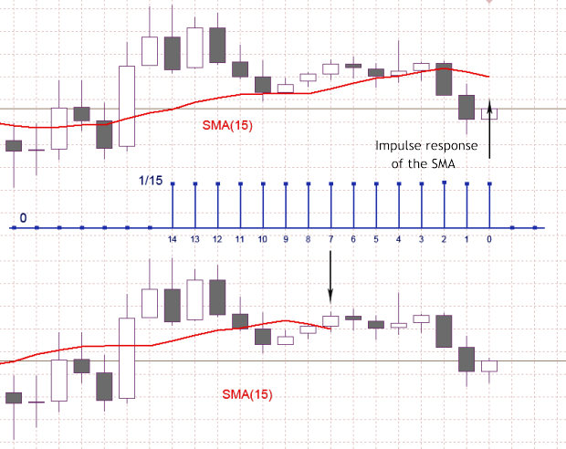
In the Figure 1 blue color shows the impulse characteristic of the low rate filter, which corresponds to the SMA (15) indicator. For the case shown in the figure, the SMA (15) is a sum of the last 15 counts of the input sequence, where each of the input counts is multiplied by 1/15 corresponding to the impulse characteristic presented. Now, having SMA (15) value calculated on the interval of 15 counts, we have to decide to what point of time we should assign this value.
Accepting SMA (15) as an average of the previous 15 input counts, this value should appear as shown on the upper chart, thus it should correspond to a zero bar. In case of accepting SMA (15) as a low rate filter with the impulse characteristic of a finite length, thus the calculated value, taking into account the delay in the filter must match the bar number seven, as shown on the bottom chart.
So, by the simple shift, we transform the chart of a moving average into the chart of a low rate filter with zero latency.
Note that in case of using zero latency charts, some traditional analysis methods slightly change their meaning. For example, the intersection of two MA plots with different periods and the intersection of the same plots with compensated delay will occur at different times. In the second case we will get intersection moments, which will be determined only by MA periods, but not by their latency.
Returning to the figure 1 it is easy to see in the bottom plot the SMA (15) curve doesn't reach the most recent counts of the input signal by the value equal to the half of the averaging period. An area of the seven counts is forming, where the SMA (15) value is not defined. We can assume that having compensated the delay, we have lost some information because of an area of ambiguity has appeared, but that is fundamentally wrong.
The same ambiguity is on the upper chart (figure 1), but due to the shift it is hidden in the right side, where there are no input counts. The MA chart loses its time binding to the input sequence and the delay size depends on the MA smoothing period because of the shift.

Figure 1. Impulse response of the SMA (15)
If all the delays occurred are always compensated when using MA with different periods, this will result in charts with a certain time binding to the input sequence and to each other. But besides the irrefutable advantages, this approach assumes areas of ambiguity. The reason of their occurrence is well known features of time finite length sequences processing, but not our reasoning mistakes.
We are facing the problems occurring on the edges of such sequences using interpolation algorithms, various filtrations, smoothing, etc. And nobody has a thought to hide the result part by its shifting.
I must admit that MA charts with a certain not-drawn part are a more correct representation of a filtering, but they look very unusual. From the formal point of view, we can't calculate the value of filter SMA (15), Shift=-7 for output counts with the index lower than 7. So is there any other way to smooth down counting on the edge if the input sequence?
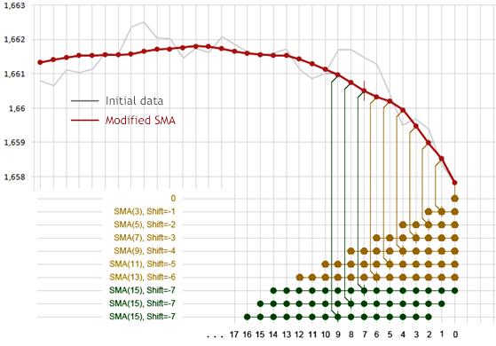
Let's try to filter these counts using the same SMA algorithm, but decreasing its period of smoothing with each bar approaching to the zero. Also, we should not forget about the delay compensation of the filter used.

Figure 2. Modified SMA
Figure 2 shows how output counts with indexes from 0 up to 6 will be formed in this case. The counts which will take part in the calculating of average value are conventionally marked with colored dots in the bottom of the figure, and vertical lines show to which output count this average will be assigned. On the zero bar no processing is made, the value of the input sequence is assigned to the output one. For the output sequence with indexes seven or greater calculations are made with the usual SMA (15) Shift =- 7.
It is obvious that when using such an approach the output chart on the index interval from 0 up to 6 will be redrawn with each new bar occurrence, and the intensity of redrawing will increase with a decrease of the index. At the same time a delay for any count of the output sequence is compensated.
In the example analyzed, we have got a redrawing indicator which is an analog of the standard SMA (15), but with a zero delay and extra information on the edge of input sequence which is absent in the standard SMA (15). Accepting zero delay and extra information as an advantage, nevertheless we've got a redrawing indicator, but it's more informative than the standard SMA indicator.
It should be emphasized that the redrawing in this example does not lead to any catastrophic consequences. On the resulting plot there is the same information as to the standard SMA, with its counts shifted to the left.
In the example considered the odd SMA period was chosen, which completely compensated the delay in time, which is for SMA:
t = (N-1)/2,
where N is a smoothing period.
Due to the fact that for even values of N the delay can't be fully compensated using this approach and the offered method of counts smoothing on the sequence edge is not the only possible, the variant of indicator construction is considered only as an example here, but not as a complete indicator.
Multi-timeframe
On the MQL4 and MQL5 websites you can see the so called multi-timeframe indicators. Let's try to figure out what multi-timeframe gives us by an example of " iUniMA MTF " indicator.
Assume we are in the lowest M1 timeframe window, and are going to show smoothed Open or Close of the M30 timeframe value in the same window, applying SMA (3) for smoothing. It is known M30 timeframe sequence forms from M1 timeframe sequence by sampling every thirtieth value and discarding the remaining 29 values. The doubts appear whether it's reasonable to use the M30 timeframe sequence.
If we have an access to a certain amount of information on M1 timeframe, then what's the point of contacting with M30 timeframe, which contains only one-thirties part of that information? In the considered case we intensionally eliminate the most of the information available and process what remains from SMA (3) and display the result in the M1 timeframe source window.
It's obvious that the actions described look quite strange. Isn't it easier just to apply SMA (90) to the complete sequence of M1 timeframe? The frequency of SMA (90) filter slice on M1 timeframe is equal to the frequency of SMA (3) filter slice on M30 timeframe.
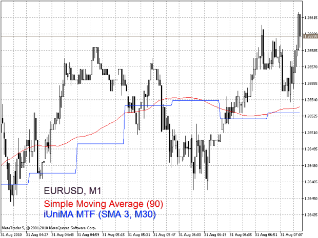
In figure 3 an example of using multi-timeframe indicator "iUniMA MTF" on the chart of EURUSD M1 currency pair is shown. The blue curve is the result of applying SMA (3) to the M30 timeframe sequence. In the same figure the curve of red color is the result obtained with the regular "Moving Average" indicator. Hence the result of applying the standard SMA (90) indicator is more natural.
And no special techniques are required.

Figure 3. Multi-timeframe indicator usage
Another variant of multi-timeframe indicators usage is possible, when an information from the lowest timeframe according to the current one is shown on a terminal. This variant can be useful if you need to compress the scale of quote displaying even more than it is allowed by the terminal on the lowest timeframe. But in this case also, no additional information about the quotes can be obtained.
It's easier to turn to the lowest timeframe and to handle all the data processing with regular indicators, but not with multi-timeframe ones.
When developing custom indicators or Expert Advisors special situations can occur, when an organization of access to various timeframe sequences is reasonable and is the only possible solution, but even in this case we should remember that the higher timeframe sequences are formed from the lower ones and don't carry any additional unique information.
Candlestick charts
In publications of technical analysis we can often meet excited relation to everything connected with candlestick charts. For example, in the article "Analysing Candlestick Patterns" is said: "The advantage of candlesticks is that they represent data in a way that it is possible to see the momentum within the data". ... Japanese candlestick charts can help you penetrate "inside" of financial markets, which is very difficult to do with other graphical methods.
And that is not the only source of such statements. Let's try to figure out whether candlestick charts allow us to get into the financial markets.
"Low", "High", "Open" and "Close" values sequences are used for rates representation in form of candlestick charts. Let's remember what kind of values these are. "Low" and "High" values are equal to the minimal and the maximal rates values on the period of chosen timeframe. The "Open" value is equal to the first known value of the rates in the analyzed period. The "Close" value is equal to the last known value of the rates in the analyzed period. What could this mean?
This primarily means that somewhere there are market rates from which values "Low", "High", "Open" and "Close" sequences are formed. «Low», «High», «Open» and «Close» values in this method of their formation are not strictly bound to the time. Besides, there is no way to restore initial rates by these sequences. The most interesting thing is that the same combination of «Low», «High», «Open» and «Close» values on any bar of any timeframe can be formed by an infinite number of variants of the original rates sequence. These conclusions are trivial and based on well-known facts.
Thus the original information is irreversibly distorted if using market rates in form of candlestick charts. Using strict math methods of analysis for rates behavior assessment by any of «Low», «High», «Open» or «Close» sequences the results are connected not to market rates, but to their distorted representation. Nevertheless, we should admit candlestick charts analysis has many advocates.
How could that be explained? Perhaps the secret is that initially the target of rates representation in form of candlestick charts was fast visual intuitive market analysis, but not applying math analysis methods to candlestick charts.
Thus, to understand how rates representation in form of candlestick charts can be used with technical analysis, let's turn to the pattern recognition theory, which is closer to usual human decision methods, than the formal math analysis methods are.
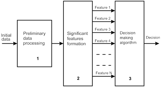
In figure 4, according to the pattern recognition theory a simplified scheme of decision making is drawn. A decision in this case can be a definition of trend beginning or ending moment and detection of optimal moments for opening a position of time moments, etc.

Figure 4. Decision making scheme
As it's shown on the figure 4 initial data (rates) is preliminary treated and significant features are formed from them in block 2. In our case these values are «Low», «High», «Open» and «Close». We can't impact on processes in blocks 1 and 2. On the terminal side only that features which are already dedicated for us are available. These features come to block 3, where decisions are made on their base.
Decision making algorithm can be implemented in software or manually by strict adherence to the specifications. We can develop and in some way implement decision making algorithms, but we can't choose significant features from analyzed rates sequence, because this sequence is not available for us.
From the point of increasing the probability of making the right decision the most crucial thing is the choice of significant features and their essential amount, but we don't have this important possibility. In this case, to impact on the reliability of this or that market situation recognition is quiet difficult, since even the most advanced decision making algorithm isn't able to compensate the disadvantages connected with nonoptimal choice of features.
What is a decision making algorithm according to this scheme? In our case, that is a set of rules published in the candlestick charts analysis research. For example, the definition of candlestick charts types, the disclosure of their various combinations meaning, etc.
Referring to the theory of pattern recognition, we come to the conclusion that candlestick charts analysis fits the scheme of this theory, but we don't have any reason to assert that the choice of «Low», «High», «Open» and «Close» values as significant features is the best. Also, a nonoptimal choice of features can dramatically reduce the probability of making correct decisions in a process of rates analyzing.
Going back to the beginning, we can confidently say candlestick chart analysis would hardly "penetrate "inside" of financial markets" or "see the momentum within the data". Moreover, its efficiency compared with other methods of technical analysis can cause serious doubts.
Conclusion
Technical analysis is a fairly conservative area. Basic postulates formation of technical analysis took part in the 18-19 centuries, and this basis reached our days almost unchanged. At the same time over the past decade, the global market structure dramatically changed during its development. Development of online trading contributed the nature of market behavior.
In this situation, even usage of the most popular theories and methods of classical technical analysis doesn't always provide us with sufficient trade efficiency.
Nevertheless, the availability of computers and interest in trading on markets being shown by people of various professions, can stimulate the development of technical analysis methods. It is obvious that today market analysis needs more accurate and sensitive analytical tools development.