Fallacies, Part 2. Statistics Is a Pseudo-Science, or a Chronicle of Nosediving Bread And Butter

Sceptic Philozoff | 13 March, 2009

Introduction

The first part of the article heading is a quotation from the post by SergNF dated April 17, 2008 14:04, https://www.mql5.com/ru/forum/108164. Well, even the most strict mathematics turns into a pseudo-science when used by a "researcher" that decides to play with attractive formulas without any practical application.

The skepticism of the quotation author, even moderated with three "smiles", is obvious. The reasons for this are quite clear: the numerous attempts to apply statistical methods to the objective reality, i.e. to financial series, crash when met with the nonstationarity of processes, "fat tails" of accompanying probability distributions, and insufficient volume of financial data. None of the existing market models can be recognized as sufficiently adequate to reality. And even if we manage to find some statistical regularities, the results of their utilization appear to be disproportionate to the efforts invested into their eduction.

In this publication I will try to refer not to the financial series as such, but to their subjective presentation - in this case, to the way a trader tries to halter the series, i.e. to the trading system. The eduction of statistical regularities of the trading results process is a rather enthralling task. In some cases quite true conclusions about the model of this process can be made, and these can be applied to the trading system.

I apologize to the readers far from mathematics for the complicacy of exposition, but obviously it is an inevitable sequence of the article contents. It seems that the promise stated at the end of my previous article, is not fulfilled. So, let's start our search.

In the article we managed to build an artificial example that vividly shows us a profitable strategy with money management (MM)rule "lot=0.1" that turns into a losing one at a geometric MM. A very regular sequence of profitable and loss trades was used there that can hardly be met in reality: P L P L P L P L P L P L ... The first question is: Why do I analyze exactly such "regular" sequences?

Loss Series: Brief Overview

The reason is simple; it is specified in the article My First "Grail":

Thus the "regular" alternation of profitable and losing trades is ideal in terms of minimal drawdowns (and maximal recovery factor). And if, like in the previous article, we manage to show that even in this ideal case (when profitable and losing trades alternate) the system turns into the losing one at a geometric MM, with the same values of mathematical expectation of profitable and losing deals, then it is sure to be even worse at a non-regular distribution of trades results.

Note: Suppose the ratio between profitable and losing trades is equal to 14:9. How should we distribute the trades in series to have minimal drawdowns? This is not an easy matter, even if we consider the MM rule "lot=0.1" and trying to prove that the series will be optimal. It is almost clear that the losses should be distributed "evenly" in the series - say, in this way:

P L P L P P L P P L P P L P L P L P P L P P L...

This is an "elementary series" consisting of 23 trades, 14 of them being profitable. After that this series repeats. It is clear that such a series has much lower drawdowns on both MM types than, for example, this one:

P P P P P P P P P P P P P P L L L L L L L L L…

It is especially vivid with geometric MM (the reasons were explained in the article). However even such a series of losses ("losing cluster") is no limit. To understand this let's refresh the basics of the probability theory. But first let's define some terms.

Terminology

This article contains a lot of terms connected with Bernoulli series and histograms that visualize various probability distributions. In order not to mix them, let us define terminology. So:

1. A full series of trades will be called here simply a series. This term refers both to the series obtained during the processing of the results of a single real testing and to the series obtained synthetically during the generation of a corresponding Bernoulli series. If the series length needs to be indicated, we will denote it like this: 3457-series (a series containing 3457 trades).
2. A sequence of successive trades of the same sign inside one series (profitable or losing trades, or, "successes" or "failures") here will be called a cluster. If the length should be indicated, it will be called, for example, a 7-cluster (a cluster of length 7).
3. A multitude of series (in this context we will mainly speak about synthetic series) will be called an array of series. The number can also be denoted: 65000-array of 5049-series (65000 Bernoulli series, each 5049 trades long).
4. When building histograms we sometimes need to take into account the clusters belonging not only to some specific series, but also to the whole array of series. The histogram name corresponds to the parameter, distribution of which is visualized. Instead of writing "Histogram of distribution of clusters with the length 4 in an array of 5000 series each 3174 long" we will denote it like this: "4-clusters in 5000-array of 3174-series».

Bernoulli Scheme: The Basics

Very often many practical tasks, in which a sequence of events is considered, can be reduced to the following scheme:

• Each event has only two results - "success" and "failure" ("win" and "loss"). The probability of "success" is p, and that of "failure" is q = 1-p.
• The probability of the event result does not depend on the history of events that preceded it.
  

This is called Bernoulli scheme (or Bernoulli trials). Our encoded colored sequence could be considered a Bernoulli scheme if we were sure in the second criterion of the definition given above.

The author thinks this is true for most trading systems. Here are some indirect proofs:

• Any information about a system Z-account, according to the opinion of those who tried to apply it for MM optimization, appears to be useless when trying to calculate the probability of a certain trade – even if the probability of a win is more than 90%;
• The efficiency of various martingale schemes, to all appearances, is also equal to zero or even negative, while it leads to inadmissible drawdowns.

That is why now it could be logical to accept that for the majority of trading systems a series of their successive trades corresponds to the criteria of Bernoulli scheme. Such a hypothesis leads to very deep consequences.

The classical formula for the probability of k wins (we can refer here losing trades as well, by the way!) in the series of n tests in Bernoulli scheme is the following (the probability of a win is equal to p):

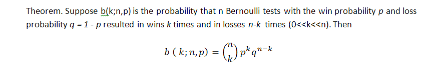
This formula shows some integral parameter of the series, number of wins, but tells nothing of how evenly these wins are distributed, i.e. we know nothing about the length of possible clusters. The search of the length of probable loss clusters in Bernoulli series is a much more difficult task; its solution is described by Feller [1]. Below are formulas for the mathematical expectation of a test series length and its dispersion with the parameters set as p (probability of a win), q (probability of a loss), r (winning cluster length) - providing we have a series of tests matching to the Bernoulli scheme: math. expectation and dispersion of return time for the winning series of r length are correspondingly equal to

It follows from the theorem that with large n the number of r long series obtained in n tests has approximately a normal distribution, i.e. with fixed the probability of the inequation

tends to

The table contains mathematical expectations for a number of typical return times.

Series length, r	p = 0.6	p=0.5 (coin)	p=1/6 (dice)
5	30.7 sec.	1 min.	2.6 hours
10	6.9 min.	34.1 min.	28.0 months
15	1.5 hours	18.2 hours	18 098 years
20	19 hours	25.3 days	140.7 mln. years

Table 1. Average return time for winning series (one test per second is performed).

Consequence 1: if we now apply (7.7) to losses and express r from the first formula, we obtain that the longest loss cluster depending on the length of test series is unlimited in length, because it grows by law of logarithm! Especially hard is the consequences for the scalping strategies (see further in the text) due to some features of such trading strategies.

Consequence 2: Limitation, considerable deceleration or, on the contrary, substantial excess of the loss cluster depending on the length of the testing series can point to the fact that the trading system does not satisfy the Bernoulli scheme. For example, if at the preassigned

n, p, q the real maximal cluster of losses is 5 items long, and the same length calculated according to the "Bernoulli scheme" hypothesis is 15, we can seriously suppose that this is a non-Bernoulli system, because trade results can appear as dependent events.

Consequence 3: if the "Bernoulli scheme" hypothesis is true, such a strategy does not differ from the scheme of tossing up an asymmetrical coin with corresponding probabilities equal to p, q = 1-p (or tossing up a sandwich with butter).

Now let's analyze a couple of "interesting" strategies from this point of view.

Scalping: "Lucky", Part 1

All, or almost all scalping systems possess a number of common characteristics:

• SL is much more than TP (typical values – 20 and 2; the point values correspond to the 4-digit quotes of EURUSD);
• p is much more than q (possibility of a profitable trade is above 80%, sometimes up to 99%);
• the number of trades is very large and can amount to tens of thousands for the period of 1 year.

We will not dwell on the third point - whether this is possible in dealing centers or not. This topic is discussed in the above mentioned article of SK., as well as in the forum. We shall assume that a dealing center does not hinder our trader by requotes, slippage, increased MODE_STOPLEVEL and so on.

A trader that has created a scalping trading system (TS) is very often mistaken about the frequency of losing trades. The roots of this illusion are traced back to the idea about the Wiener character of closing price processes and the true character of the Einstein formula for the Brownian motion: "if we set SL=20, TP=2, the possibility of stop-loss triggering is (20/2)^2=100 times lower than the possibility of TP hitting; therefore such a TS must be profitable". The delusiveness of this conception is in the fact that this process is not the Wiener process and corresponding possibilities actually differ in much less than 100 times!

Exactly in this case the "Bernoulli scheme" hypothesis is quite probable - just because the scalping trading strategies often try to use random peculiarities of the process and of its filtration accepted in some given dealing center.

Now let's take the parameters of the trading strategy known to us under the name "Lucky" (https://www.mql5.com/en/code/7464). In its original form (in the same section, Lucky_new.mq4) this EA is only a toy, because there can hardly be a dealing center that accepts the opening of several hundreds of trades per day with the mathematical expectation of profitable one around one-two points. However one can slightly modify the code and set more strict requirements to the TP level and still sometimes get quite satisfactory balance/equity curves. The code of the modified EA (taking into account the restrictions on the number of trades opened at the same time, which is in this case equal to 1; see explanations below) is attached to this article.

The main advantage of this EA is that it executes a huge amount of trades and gives a rich material for statistics - this will be proved further. Now we are only aimed at finding evidences confirming or refuting the hypothesis: "the trade results agree with the Bernoulli scheme". For those who like to argue about the non-random character of market movements, I will specify: I do not doubt that quote movements are not always random. I will not assimilate market (exactly market!) to the coin tossing up a la Bachelier; I am interested only in the statistics of trade results - and nothing else. Further you'll see that some sets of external parameters are intentionally chosen as "losing" - only for checking the hypothesis stated.

Here are the results of the first test:

Both first external variables have the same meaning as in the original code, the third one is the value of profit in points, which an order should exceed to initiate the take profit event. Let's estimate, according to (7.7), the mathematical expectation of the minimal test series necessary to meet the 11-cluster of losses (p=0.8937, q=0.1063, r_loss=11):

N_loss = 1 / (p * q^r_loss) – 1 / p ~ 57 140 275 804

Here is the analogous estimation for the math. exp. of the test series length for meeting the profitable 141-cluster:

N_profit = 1 / (q * p^r_profit) – 1 / q ~ 71 685 085

Well... As we know, the real length of series is equal to only 16255 trades, and not tens of billions or millions. Such a huge excess of the real series length is the sign that for this TS the Bernoulli scheme hypothesis hardly works directly. Maybe here is an influence of a factor that we didn't take into account?

Bernoulli Scheme: An Interesting Result

There is such a factor: an expert adviser (EA) can open much more than one trade at a time: in the second hundred of trades (orders 158…163) it opened 6 trades in succession (and it closes them in "heaps" as well)! This "multiplication factor" is probably responsible for the substantially increased cluster lengths as compared to the expected ones: if the market is in flat with a substantial volume, the EA starts to open a lot of trades almost on each tick. However, due to its work character, because of the flat market and small size of the take-profit as compared to the stop-loss, most of them, if not all, will be closed profitable. On the other hand, if a strong directed motion starts, the EA will open many unidirectional trades in the direction opposite to the market movement - and finally most of them will be closed losing and also "massively".

Let's conduct simple computations. We take both formulas for math. exp. of the full test series length from the previous paragraph. Here r_loss_real, r_profit_real are the real lengths of maximal losing and profitable clusters correspondingly. While the obtained N_xxxx values are rather large, lopping off the second terms (1/p and 1/q) will practically make no error, if we divide these equalities by each other termwise:

N_loss / N_profit = q * p ^ r_profit_real / ( p * q ^ r_loss_real ) =

p ^ ( r_profit_real – 1) / q ^ (r_loss_real – 1)

Let's find the logarithm and simplify:

ln( N_loss / N_profit ) = ( r_profit_real – 1 ) * ln( p ) - ( r_loss_real – 1 ) * ln( q )

Now let's mark that if the tests are governed by the Bernoulli scheme, and the lengths of longest clusters and both possibilities p and q are not very small, then N_loss and N_profit values should be approximately equal. So we obtain an interesting approximate correlation:

( r_profit_real – 1 ) / ( r_loss_real – 1 ) * ln( p ) / ln( q ) ~ 1 (*)

And if we rewrite it in another way:

p ^ ( r_profit_real – 1 ) ~ q ^ ( r_loss_real – 1 )

the meaning of the correlation (*) becomes clear: in the Bernoulli TS (at a rather long test series and not too small p and q possibilities) the possibilities of two maximally long clusters ("wins" and "losses") are practically equal. Actually, this principle can be applied to any other TS that are non-Bernoulli as well, but the (*) correlation form is specific for the Bernoulli scheme. This correlation can be called a rough test of a TS for "bernoullity".

Scalping: "Lucky", Part 2

Let's exclude the multiplication factor: set the limitation for the number of orders opened at the same time to 1. While the number of orders is diminished several times for the same time-period, we will extend the range of testing and set it from the 1st of January 2004 to the 4th of April 2008. Below is the table of results and some calculations (BS is an abbreviated form of the "Bernoulli scheme" (see analysis below); the first "+" denotes a good correspondence to the Bernoulli scheme for profitable clusters, the second one for losing clusters, "-" is a refuted hypothesis "The system satisfies the BS", "0" means doubts in its correctness):

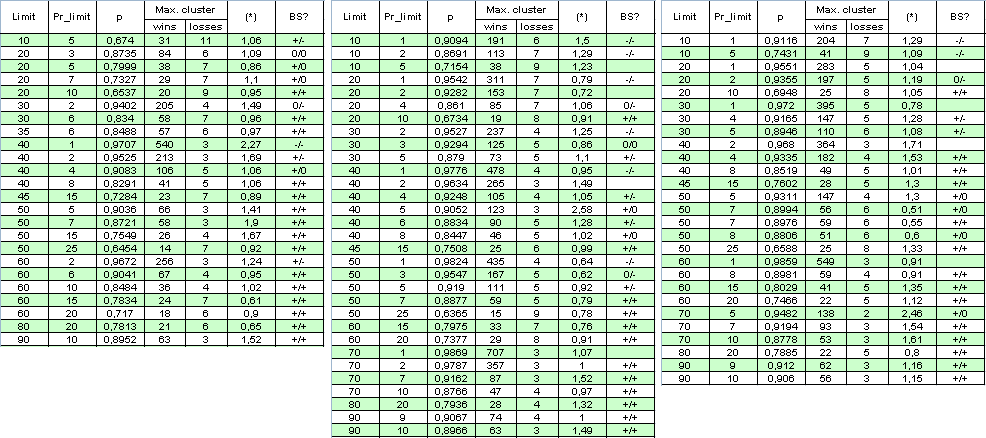
The author apologizes for the large size of the table, to get the full picture. The parameter (*) appears to be insufficient for deciding on the "bernoullity" of the system, because sometimes even when it is close to 1, the system can hardly be referred to the Bernoulli scheme.

P.S. Even despite the fact that the multipliers in (*) sometimes do deviate quite far from 1, the (*) values are still close to 1. For example, if Limit = 40 and Pr_limit = 1 in the second column, we have:

( * ) = ( 478 - 1 ) / ( 4 - 1 ) * ln( 0.9776 ) / ln( 0.0224 ) ~

477 / 3 * ( -0.02265 ) / ( - 3.7987 ) ~ 0.95

This fact by the way acknowledges another conjecture: even if the system Bernoullity hypothesis is deferred, the dependency of the trades here is "almost the same" for profitable and losing ones.

Criterion of Correspondence of a Trading System to the Bernoulli Scheme.

Description of Script Operation

How can we divide more reliably testing results into two groups - Bernoulli schemes and "non-Bernoulli-schemes"? We can try several methods, but the simplest one, in my opinion, is the following: if we generate a lot of Bernoulli series with parameters corresponding to those really detected during testing, in case of the system's "Bernoullity" the probability distribution function (p.d.f.) of the cluster length should remain nearly unchanged. This fact obviously results from the assumption about the invariability of the win probability and the independence of trades.

Unfortunately, the theoretical function of distribution of win/loss clusters according to their length is unknown to me. Above, I included some formulas allowing to estimate math. exp. of winning cluster number in the test series depending on its length and probability of win (see (7.8) above). For this purpose Feller ([1]) offers a special method following from the theory of recurrent events, to which clusters belong. On the first sight this method does not fully suit a trader's understanding of the "winning series" term, but this method substantially simplifies the theory itself, so that the identification of the "r-cluster registration" event does not depend on the future ([1], page 302):

On the other hand, for a trader the numbers of winning clusters ("win series" by Feller) in the indicated row (WWWWLWWWWWW) will be the following: first 4-cluster of wins, then, after one loss, 6-cluster of wins. There are no "completed" clusters of the length 1, 2, 3 and 5 for a trader, though there are such according to Feller. This extract from [1] is published here only to indicate the difficulty of the problem. Thus, we will just generate a large number of Bernoulli series and detect series in them, which correspond to the understanding of them by a trader (15 wins at a row ending by a loss are not 15 registrations of 1-cluster, or 5 registrations of 3-cluster, as according to Feller, but it is only one registration of a "true" 15-cluster). For checking the series for "bernoullity" 1000 Bernoulli series are enough.

According to this idea, first a script was written allowing to upload the sequence of results of real trades into an array and then get data for drawing a histogram of cluster length in MS Excel. This script also contains the functions which generate Bernoulli series and prepares the data to make histograms in MS Excel. I wouldn't like to insert the script code into the article; instead I will give general comments for the code. The script is attached below. The tester report file should be first placed in the directory experts\files\Sequences\, and its name should be moved into external script parameters.

At the beginning, on the basis of the tester report file, with the help of the readIntoArray() function, the binary results of trades (1 or -1) are entered into a global array _res[]. To understand the operation let's illustrate our explanations using a small array. This function operation finally results in, for example, the following array _res[] (the number of trades, i.e. the series length, is 50):

1,1,-1,-1,1,1,1,1,1,-1,1,1,1,1,1,1,1,-1,1,1,-1,-1,-1,-1,1,1,1,-1,1,1,1,1,-1,1,-1,1,-1,-1,-1,1, 1,-1,1,1,1,1,1,1,1,1

After that the function formClustersArray( int results[], int& sequences[], int& h, int nr ) calculates the lengths of clusters and then, depending on the global parameter _what, which defines what we are interested in - profits or losses, writes down lengths of series into the array sequences[] (actually into the global array _seq[]). Let's count clusters in this array:

2,-2,5,-1,7,-1,2,-4,3,-1,4,-1,1,-1,1,-3,2,-1,8

Negative values refer to the losing clusters. It's clear that the sum of all absolute values of the numbers is equal to the series length, 50. Suppose we are interested in losses, i.e. _what = -1. Then the array _seq[] will store only negative values, but with the "plus" sign:

2,1,1,4,1,1,1,3,1

After that the array _seq[] is processed with the purpose of building the array _histogramReal[]. Now we need only to calculate the quantities of 1-, 2-, 3- etc. clusters and write them in a sequence into the array. As a result the array _histogramReal[] will contain the following values:

6,1,1,1

This means that our series contains 6 losing 1-clusters, 1 losing 2-cluster, 1 losing 3-cluster and 1 losing 4-cluster. Further the latter array is written in the output file. The file is not closed, because we need to write into it analogous "histograms" of synthetic series of tests according to the Bernoulli scheme.

When forming "synthetics", the key function is the generator of a single test according to the Bernoulli scheme. Despite of this simple code, it operates quite well: no "edge effects" responsible for the distortion of the regular distribution of results in the segment [0, 32767] were observed.

// generates a single Bernoulli test (+-1 with different probabilities)
int genBernTest( double probab )
{
   int rnd = MathRand();
   if( rnd < probab * 32767 ) return(  _what );
   else                       return( -_what );
}

After a single call of MathSrand( GetTickCount() ), this function is called as many times, as there are real trades in the testing period (_testsTotal). Then, when we have the generated Bernoulli series, the results are correspondingly processed by cluster counting and "histogram" constructing functions. These actions are responsible for the creation of one histogram corresponding to one testing (the function genSynthHistogr( int& h, int nr ) ). And finally the last function is called in the loop, so that in the result the array of Bernoulli series is generated, histograms for them are formed and they are written into an output file.

Now we can open this file in MS Excel, build necessary diagrams and draw conclusions about the correspondence of the system to the Bernoulli scheme. Numbers in the file lines have the following meaning (the table is cut, and we don't show here the data on 5-clusters and further):

No of test series	Length of max. cluster	Number of 1-clusters	Number of 2-clusters	number of 3-clusters	Number of 4-clusters
1	9	1639	1058	724	440
0	11	1649	1044	688	478
1	8	1681	1093	675	458
2	13	1628	1067	701	461
3	7	1616	1039	726	474
4	12	1601	1054	699	465

The first line of the file (green) shows the result of real testing, and lines below correspond to synthetic test series, with the number starting from 0.

And, finally, the last stage - estimation of real testing results for the correspondence to the Bernoulli scheme: from the synthetic Bernoulli series corresponding columns are chosen to construct a histogram of the necessary length clusters. For example, to construct a histogram of winning 1-cluster quantity distribution, we should take the third column (1649, 1681, 1628, 1616, 1601….); the total quntity of such numbers is equal to the quantity of synthetic Bernoulli series). For winning 2-clusters we take the fourth column (1044, 1093, 1067, 1039, 1054…), and so on.

Such histograms are constructed according to the method described by Bulashev [7], and then we check the Zero Hypothesis about the equality of the number in the real test to the estimation of the average in synthetics series. The preaccepted level of significance for Hypothesis Zero, "Real number equals an average for synthetics", is equal to 0.05 (it refers to approximately two standard deviations).

First Results

Let's start the script on Lucky testing results at the parameters 3, 20, 10. The script parameters: _what = 1 (profitable clusters), _globalSeriesQty = 5000. Parameter (*) in the large table is equal to 1, i.e we can expect that the script operation results should show the correspondence to the Bernoulli scheme. We'll show here only the file records corresponding to the direct checking of the Zero hypothesis for cluster lengths 1-6 (they are slightly amended into a table form for easier perception):

// The first line of the file is results of the real test made in the tester. The two first figures are the number of series and the length of a maximal cluster.

1,20,1639,1058,724,440,271,212,137,91,62,30,26,22,5,7,1,4,1,0,1,1,

…

// End of file (partially):

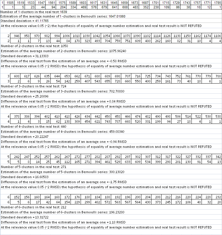
In each of 6 two-line tables the upper line corresponds to left values of histogram intervals, and the lower one to the number of Bernoulli series (out of 5000), in which the numbers of clusters of the given length were inside these intervals. Below the same is visualized graphically (the number of profitable r-clusters in Bernoulli series provided the total number of series is equal to 5000):

Abscissas of red spots correspond to the numbers of clusters obtained in the real test. The same script for losing clusters (_what = -1) at the same parameters also gives quite a good picture - with the discount for the reasonable length of losing clusters: as soon as the number of intervals calculated according to recommendations in [7] starts to exceed the spread of data in synthetics, the construction of histograms with the set number of intervals is impossible. Nevertheless, formal zeros in the script report should not scare you, because all necessary parameters can be calculated without a histogram. At the preset parameters only for the 3- and 7-clusters the zero hypothesis was rejected. As the main criterion for referring a tested system to the Bernoulli system a very doubtful criterion of the fuzzy type was chosen. Let's consider the principle of decision making on the example of the script operation results for losing clusters:

The difference of a real test from the estimation of an average = -0.37 SD (standard deviation)

The difference of a real test from the estimation of an average = 0.95 SD

The difference of a real test from the estimation of an average = -2.04 SD

The difference of a real test from the estimation of an average = -0.45 SD

The difference of a real test from the estimation of an average = 0.36 SD

The difference of a real test from the estimation of an average = 1.13 SD

The difference of a real test from the estimation of an average = 3.27 SD

The difference of a real test from the estimation of an average = 0.11 SD

The difference of a real test from the estimation of an average = 0.46 SD

The difference of a real test from the estimation of an average = -0.47 SD

So, here is the main criterion:

• If the average of figure modules does not exceed 1.5 (here it is 0.96),
• the average of figures is not more than 1.2 by module,
• the number of outlayers (here they are bold and correspond to the difference exceeding 2 SD) does not exceed 20% of their total quantity,

a system is considered "surely bernoullian". If the corresponding "critical" figures are 2, 1.5 and 30%, the system is "doubtfully bernoullian". If the figures exceed these boundaries, the hypothesis is refuted. I consider the second point reasonable, because the deviations shouldn't be of mainly one sign.

Statistical criteria of the correspondence to the Bernoulli scheme are unknown to me, and that is why I had to think up such a criterion. The results of such an improvised decisive criterion are given in the script operation report file. An interested reader can offer a more reasonable decisive criterion.

For this case we can "conclude for sure" that the Lucky_ system with parameters 3, 20, 10 really comply with the Bernoulli scheme, i.e. with the scheme of a bread-and-butter thrown randomly.

Now let's take one of the "worst" cases and conduct the same calculations at the number of Bernoulli series equal to 1000; the parameters of Lucky are 5, 10, 1. Let's consider profitable 1-clusters:

Even on the first histogram everything is completely different: real test results (619 1-clusters) do not conform with the "synthetics" with the same length of test series and the same win probability. Therefore, the trades are not independent.

Note that similar estimation tests with many other sets of parameters of a large table allow concluding that the Bernoulli scheme ("throwing up a bread-and-butter") is more a rule than an exception. Besides, there are cases when for some group of trades (e.g. "profitable trades") the Bernoulli scheme is satisfied, and for another group it is not. This does not hinder using this model at least partially for getting useful information, which will be discussed later in this article. And the last thing: the decisive criterion is not so reliable on losing clusters because of the insufficient amount of statistical data, but I applied the script for them also - just for obtaining the full picture.

"Universum" System: Bernoulli Scheme Again!

Now let us take absolutely different system for our study - "Universum"; its source code is posted at https://www.mql5.com/en/code/7999. The author claims that the system operates at the formed bars, that is why "all ticks" testing is not necessary. The starting balance, at which the system can gather trade statistics for the period 2000.01.01 - 2008.04.04, was set equal to about $10M. The first opened lot is 0.1. Actually the three parameters changed are p, tp, sl. No multiplication presents, so the study is easy:

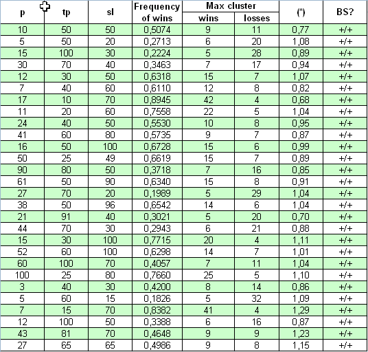
See, here the conformity of (*) parameter with 1 is much better, than in the previous case: (*) values slightly differ from one. The check with a decisive criterion also shows that in all cases, at quite wide parameters range, this TS complies with the Bernoulli scheme.

Preliminary Conclusions

Ralph Vince in [4] offers another procedure of test series checking for the correspondence to the Bernoulli scheme. This is the calculation of Z-score and test of trade results for a special correlation (autocorrelation of a source row and a row shifted by one). I do not feel that his procedure gives much more significant results than the one described above (where the deviation of clusters numbers with different length in real series is checked vs. model series). True, the offered decisive criterion is rather free and needs some substantiation. Besides, as I have noted earlier the reliability of this check at a short length of the maximal cluster isn't high (for Lucky_ these are usually losing series tests). However, in my opinion, though this decisive criterion needs more extensive calculations, it is better to cover the specific character of test series in the context of their conformity with the Bernoulli scheme. This question needs further studies and, of course, is not closed yet.

Nevertheless, expectations have been proved: in most cases, at quite different sets of external parameters, the trade series do correspond to the Bernoulli scheme, and the deviations from the Bernoulli scheme almost always result from the systematic exploiting of regularities that are characteristic of quotes filtering process and more often inherent to the systems with the small value of Pr_limit. This is especially evident in the large table with Lucky_ check results.

Vince notes that if the empirical check of serial correlation or Z-score test revealed the dependency between trades, then the system is sub-optimal, and the dependency should be explicitly included in the TS, to lower it in the test results and increase the TS optimality. Thus, putting the testing results of the two systems off, we should admit that the "Universum" system is generally more optimal than the "Lucky" system. However, this does not justify the MM used in Universum.

How to Possibly Use the Bernoullity of the System?

1. What do we know now?

Knowing beforehand that at least in some cases the sequence of trade results expressed by 1 ("success", i.e. profit) and -1 ("failure", i.e. loss) is the Bernoulli one, we get an adequate model of this process. Now we know enough about this process, because actually this is a modification of a usual Brownian motion with a drift. P. Samuelson has introduced geometrical (or, as he called it, economical) Brownian motion in the financial theory and practice ([6]):

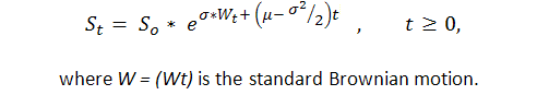
Thus, we can apply strong results of theoretical studies of the standard Brownian motion (arcsine laws, for example) to the balance curve. However, the Brownian motion theory us quite complicated and can be understood only to the close number of people with a solid mathematical education in stochastic integration.

The second approach is to refuse from the highly theoretical computations, conduct direct program generation of long Bernoulli series, and then transform these into balance curves for "testing MM 0.1 lot". Here we need to know only average values of profitable and losing trades and the win frequency p. Even several hundreds of such series (for example, 1000-array of Bernoulli series) can give us quite a good idea of what a strategy which complies with the Bernoulli scheme is able to.

It is important to understand clearly that such a synthetic testing is a good alternative to a tiresome Pardo testing ([5]): if we are truly able to validate the Zero Hypothesis ("trade succession is bernoullian" is not refuted), it can provide us with enough information about the system substantially different from the one given by the walk-forward-analysis described in [5]. Of course the balance curves can differ much from the curve obtained by the real testing.

***********

Generally, nothing hinders the implementation of such an approach because such a testing is performed on a computer for several minutes; as a result we get wide information that can be thoroughly analyzed. Unfortunately, the article volume does not allow posting all results. Here are several charts for Lucky_ with parameters 4, 70, 10 in the same testing period as in the table. The task of generating synthetic Bernoulli schemes is much easier that tasks performed by the above described script; so means of MS Excel are quite enough.

Real test on 0.1:

The following parameters from the report are important to us; we will set them when generating Bernoulli series and transforming series into balance change curves:

Frequency of profitable trades (p)	0.8765
Average win. trade	11.71
Average loss trade	-73.73
Total amount of trades	5904

Synthetic curves of balance changes based on Bernoulli series:

We see, despite the fact that series were generated at identical input data, the integral balance result at the end of the testing period are considerably different from series to series - from a small loss (blue line) to large profit (red line). I must admit, I didn't manage to generate a series with an evidently falling balance (though, I wanted to achieve such a chart and made about 200 attempts). Perhaps at a large number of series this could be achieved. But it seems such a case is not typical of this strategy. Besides, in none of the series I saw drawdown more than 2500 points.

Now let's consider a couple of isolated results connected with the estimation of some parameters of a strategy that complies with the Bernoulli scheme.

2. Estimation of a maximal losing cluster exceeding report values ("black swan")

Having received evidences of the system's bernoullity, we can realistically estimate the maximal length of a losing cluster that can await us at the same amount of trades as in real testing. Here we can just generate a lot of Bernoulli series and then estimate the chances of a real "black swan" (see [2, 3]), i.e. such an event, for which we'd never be able to estimate the possibility based on the testing results only, because it simply hasn't happened in the testing period. It's just this probability-theoretical model that we can gather the necessary statistics for in any volume we need.

Let's use trading results of all the same Lucky_ system with the parameters 4, 50, 7:

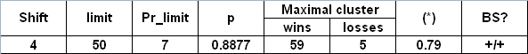
According to the report, the length of the maximal losing cluster is equal to 5. Now let's set a very large number of Bernoulli series, 65000, with the parameter _what equal to -1 (losing clusters), and then apply our script to the tester report. Let's find the longest line (the 1st number is a # of Bernoulli series, the 2nd one is the length of the maximal cluster, and then go numbers of clusters of each length):

26001 9 1030 136 13 4 0 0 0 0 1

See, the length of the maximal loss cluster can be much longer than 5 (here it's 9)! Maybe this is too rare an event? True, it is very rare: it was met only once out of 65,000 series, so its appearance in a real test can be considered as almost disappearing, taking in account "the ergodicity hypothesis" (see a bit later). Nevertheless this frequency estimation is very unreliable; therefore one cannot rely on it: this series could occur, for example, among only 20 Bernoulli series. As a result, if we didn't know the statistic criteria of reliability estimation, we'd erroneously consider that this estimation had high probability.

In the version as I offer it, "the ergodicity hypothesis" is the following: the probability of an event in the "synthetic tests space" (based on the adequate model of the event) is approximately equal to the probability of the same event in the time space, i.e. for the real trading - providing the number of trades in the real test is equal to that in model tests. It is considered, of course, that the sequence of trades results in the real tests is stationary, like the Bernoulli scheme. At a large amount of trades this statement is not so far from being true, because the only source of nonstationarity here can be, probably, the so called "win drift" distributed according to the normal law and described below.

Below is the table of losing clusters numbers in the 65000-array of Bernoulli series:

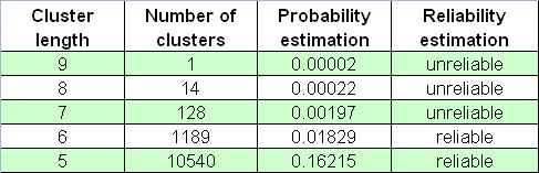
We still should not forget about "black swans" that come exactly when you do not expect them.

In contrast to the above calculations we can use estimations for "black swans" of a contrary character, namely profitable clusters of the increased length. We remember that the real testing shows that the length of the maximal profitable cluster is equal to 59. Carrying the analogous modeling for 65,000 model series, we again find the longest line in the script report:

44118 153 115 117 111 87 70 71 52 51 50 40 36 42 42 34 20 32 15 20 20 13 10 11 12 8 5 7 3 5 4 2 2 6 7 0 2 1 2 1 1 5 0 0 1 0 0 0 0 0 0 1 0 0 2 0 0 0 1 0 0 0 0 0 0 0 0 0 0 0 0 0 0 0 0 0 0 0 0 0 0 0 0 0 0 0 0 0 0 0 0 0 0 0 0 0 0 0 0 0 0 0 0 0 0 0 0 0 0 0 0 0 0 0 0 0 0 0 0 0 0 0 0 0 0 0 0 0 0 0 0 0 0 0 0 0 0 0 0 0 0 0 0 0 0 0 0 0 0 0 0 0 0 0 1

This is a model series #44118, with the maximal profitable cluster length equal to 153 trades (2nd figure in the list), approximately 2.6 time longer than the maximal cluster in the real test! However, the statistically significant estimations of clusters frequencies may be obtained at their length starting from about 80 (the probability estimation of the series is 0.0088) and lower, and 80 is much more than 59. The quantile of ½ order (the value of cluster length at which the integral distribution function obtains the value of 0.5, i.e. such a value, by which the distribution is divided in two parts equal in area under the function of probability density distribution) for profitable clusters is about 62, i.e. a little more than 59. The histogram of maximal cluster length distribution on Bernoulli series array is included here for your reference:

Of course, the "black swan" term is used here not very carefully, because as of Taleb this seems to be an event the probability of which is incomputable. Nevertheless, we may note that, judging by empirical data only (testing report) and using no theoretical models, we would hardly make any statistically reliable conclusions about the probabilities of losing 6-clusters or profitable 80-clusters, i.e. for the events we don't meet in the report!

3. "Failure drift": An Unfavorable Deviation of Failure Probability from Empirical Frequency.
Approaching Apparatus, Attempt No. 1

At the large amount of tests in the series by Bernoulli scheme (about several thousands or so) the failure frequency f slightly differs from the failure probability q and obeys the "correct" normal distribution with a little variance: the law of large numbers (here Laplace theorem) is still effective. Nevertheless, f can also drift, and for scalping strategies with a very small mathematical expectation of a trade such a drift can be critical and is able to turn the system into the losing one for the whole testing interval. We now have the facilities enough for the statistical estimation of chances of such a drift - if there is an evidence proving that the Bernoulli scheme "works" in this case.

Unfortunately, the EA Lucky_ even limited in its possibilities till one trade for a fixed time gives too much statistics.

For a serious strategy developer this is more an exception than a rule, because one usually has to make snaky conclusions based on the test results containing several hundreds or even dozens of trades (see explanation below). The increase of statistics volume appropriately leads to the corresponding lowering of the width of Gauss distribution and considerably lowers chances for large deviations from its central value.

As an example let's consider Lucky_ with the parameters far from favorable for the EA: 4, 80, 20, on the lot 0.1. First let's conduct its testing for the full time interval ("interval A") – from January 1st, 2004 to April 4th, 2008 (EURUSD H1). Here is the balance chart given by the report:

We see the to be far from amazing. After checking the sequence of trades with our script (on 1000 model Bernoulli series) we find that the full trade series can be considered corresponding to the Bernoulli scheme - both for profitable and losing clusters.

Let's notice the parameters of average trades:

Average profit trade

21.71

loss trade

-83.32

Now, suppose we tested the EA only for a short period from 2005.10.21 to 2007.06.07 ("interval B"), where the strategy shows a stable growth. The chart is below:

Here are the results of average trades:

Average profit trade

21.69

loss trade

-82.94

In average the trades have changed very slightly; therefore they may be considered approximately invariant, irrelevant of the strategy profitability for the period of testing. Actually we could see this earlier, taking in account that the trades are closed only after they reach a certain profit/loss level set by the strict external parameters.

The second express check for bernoullity (1000 model series) again confirms its compliance with Bernoulli scheme. Now let's apply our script with a large number of Bernoulli series (65000) to the results of the short testing time (interval B), and then import the results of 65000 Bernoulli model series into MS Excel to build the histogram for the distribution of the profitable trades ratio:

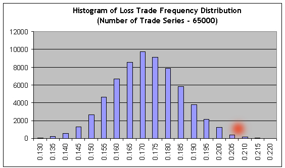
It is obvious that to achieve the nonprofit, the frequencies of profits and losses should relate inversely to the ratio of their average values: r = 21.69/82.94 = 0.2615. Consequently, the frequency of loss trades should be equal to f = r / ( 1+r ) = 0.2073. We see that this value (see the red spot) is located far in the area of the right tail, where the sum of bars to the right is about 0.3% of the sum of all histogram bars, i.e. nonprofit/loss chance probability is about 0.003. Approximately the same value is obtained at the direct use of Laplace theorem.

Something is wrong in Danish Kingdom: the report data on interval A tell us that in the first half of A, prior to this growth interval, the balance was falling almost the same rapidly, and the falling period is not shorter than B as for the number of trades. If we estimate the probability of approximately the same interval of falling balance (stable loss) on the basis of our testing data of the interval B, it will become vanishing (because the boundary frequency f will be shifted even more to the right), and this seems to be contradictory to the experimental data.

Probably, the problem is that such a long series of trades with the profitability corresponding to the interval B is a very large deviation: the testing from January 1999 to the beginning of May 2008 shows that this strategy is neither profitable nor losing:

The mathematical expectation of a trade is only 0.17, and the "natural" frequency of losing trades is approximately equal to the earlier calculated f (0.2073) and makes up 0.2054.

It is clear that estimations of probabilities based on the statistics of rare events (the frequency of losing trades on the interval B is equal to 0.1706, and it differs from "natural" one in about 2.8 "sigmas" in the favorable direction) cannot be reliable enough. But we cannot know the "true" frequency for sure. Still, can the "failure drift" notion bring benefit to us?

4. "Failure drift": Probability Estimation of Short-Term "Shock" Drawdowns.
Approaching Apparatus, Attempt No. 2

Apparently, we can - if we set reasonable, not extreme targets corresponding to the "tails" of distributions. Let us put the task this way: suppose we have testing results for the interval B. We are sure that this is Bernoulli scheme, and the mathematical expectation of profitable and losing trades practically do not depend on what is happening to the balance. Based on very optimistic (actually false!) estimations of loss probability, let's try to estimate our chances for short but deep "shock" drawdowns. Exactly such drawdowns have the most devastating effect on a trader's psyche, because after that a trader starts talking mystical phrases like "the market has changed" or even "has become a command one".

I should add here that Laplace theorem would not be of great help here, because the value n*p*q contained in its formula will be small, about 10 and lower (this corresponds to approximately several dozens of trades). The main idea in the basis of this calculation is that in very short trade series the frequency of losses can sufficiently differ from the "true" one, i.e. from the probability: the distribution of loss frequency is spread widely because of the small number of tests.

Note that the estimation of a short-term drawdown is the task that differs much from the problem of estimating the maximal length of a losing cluster, because a drawdown does not necessarily consist of losing trades only. Let's use our script to generate 65000 series of the length 40 at a "very favorable" frequency of losses 0.1706 ("interval B"), and then build the histogram like the one in Approaching Apparatus, Attempt No. 1:

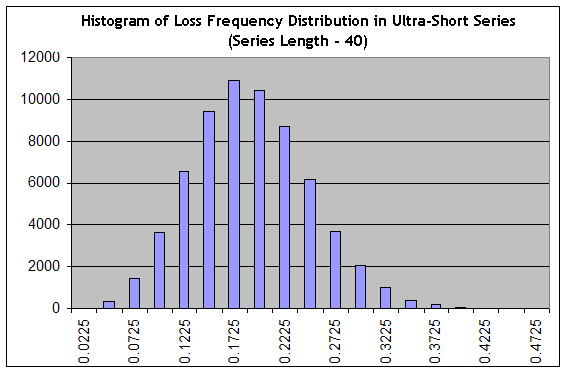
We see that the set-up has changed crucially: from a sharp one the distribution turned to a smooth one, i.e. its "relative width" has increased. The probability that in 40-long series we will obtain something in the range from practically profitless trading (f.e., at the frequency of losing trades equal to 0.1975 an average trade makes 0.25 points) to a sharply losing trading (at the frequency of losing trades 0.3000, the estimation of a trade math. exp. in this series is equal to 0.7*20-0.3*80=-10 points), is equal to the sum of columns from "0.2225" column and to the right of it, which is about 34% from the total sum of columns (65000). All the same, this is an optimistic estimation, because the distribution peak is at the "optimistic" frequency 0.1706!

Calling the ergodicity hypothesis to the mind, which is putting a bridge between the probability distribution and the trading space, i.e. the real time space, we obtain that at least 34% of the trading time the system will not make profit or lose at the average. This figure correlates quite well with the data in [4], according to which a Bernoulli system remains in drawdown approximately from 35 to 55% of all the trading time.

Pay attention to the fact that the actual probability to meet a shock drawdown does not strongly depend on the initial "favorable" frequency, no matter how attractive it looks like. This is the characteristic feature of the system, which is connected with its bernoullity, and this event can be smoothed only by the improved ratio of average profitable and losing trade results.

By the way, exactly these estimations based on the generation of ultra-short series allow often very reliably to sift away the testing results of quite a "profitable" system with only dozens of trades at the testing interval: despite the quite a positive "mathematical expectation" of a trade, at such a little number of trades the "shock" drawdowns are inevitable, in case of the system bernoullity.

Conclusion

In spite of the fact that we like to build the logical constructions proudly called "Mechanical Trading Systems", we often do not realize how much randomness they contain - including the one that we do not meet in the testing results ("black swans").

As the results of successive trades expressed in the binary notation ("success" or "failure") quite often comply with the Bernoulli scheme, they do not have any expressed difference from the tossing up of bread and butter. Of course, this does not mean that profitable systems are impossible: a strategy can be both profitable and robust, even if it ideally complies with the Bernoulli scheme. This clearly results from the idea that if both the probability of a profitable trade and its math. exp. are stably higher than those of a losing trade, the strategy is obviously profitable.

A reader who at least sometimes is able to "communicate" with mathematics as a "relative" should understand the benefit of models quite well - even if they are far from being deterministic. The main value of the models that are adequate to the real statistical phenomenon is that they allow obtaining a valuable knowledge about the universe - i.e. the information that cannot be obtained right from scant experimental data. In this case the value of Bernoulli scheme is considerably higher because of extreme simplicity of its generation and absence of "thick-tailness" in key probability distributions.

Let us close this article by a very hard question: probably, the analytical part of most TS is useless, and the main efforts are to be invested in the efficient and well-grounded money management methods ("Analytics is nothing, money management is all!"), aren't they?