Principles of Time Transformation in Intraday Trading
kamal | 21 August, 2007
Introduction
Statistical homogeneity of observations always plays an important role in analyzing previous price movements. When such homogeneity takes place, it is possible to study deeply the process properties for the revelation of regularities that contribute to building a trading system. But it is a well known fact, and it will be proved later that even at the first approaching the process of exchange rate is non-homogeneous, namely there is a heterogeneity, connected with the activity of different trading sessions: American, European, Asian and switch between them.
I will dare say that few of new systems developers and not all "experienced" ones ever think that even the simplest indicators of the moving average type, bound to time, are actually different units in different parts of the day. Undoubtedly there are systems, formulated in terms of prices, not time. A typical example - systems based on renko and kagi methods, but they are minority. But, I will repeat, the majority of them are bound with time, usually indirectly - through indicators.
All the above obviously refers only to intraday-systems. For larger timeframes, even if there is seasonality, it is not so apparent. And in intraday trading it is essential and very often leads to the fact that the system shows different profitability in different times. Let us dwell on the factors, causing such effects, and the ways to overcome them.
Theory
From the point of view of accidental processes statistics, the process of price change at a first approximation is usually treated as a certain diffusion kind, i.e. transfer of a substance or energy from an area with high concentration into an area with low concentration. It is well known that the time transformation brings continuous martingales to a relatively easily arranged Brownian motion.
Not dwelling on the question, whether the process of price change is a diffusion or martingale, let us remark that nothing hinders switching in the same way from the process of time transformation to something arranged in a simpler way, namely to a process statistically homogeneous in time. For this purpose it would be natural to use bars not with time division, but simply with a fixed number of ticks, i. e. a bar contains not 60 minutes but for example 1000 ticks.
Such time in theory is called operational and is natural for the process of time transformation. In this case the process has a statistically constant average deviation, which enables to detect more clearly the forming market atmosphere and efficiently separate them from accidental fluctuations. And note that using common indicators would be not only possible, but also much more homogeneous. But unfortunately MetaTrader 4 does not contain such an option yet. So, we will use another method - rearranging the system with an allowance for time. Below are the examples of amended indicators. But first let us analyze the heterogeneity we are talking about.
Statistical Data
A chart of exotic currency pairs vividly shows that the activity in the market is reduced in a certain part of a day. For example:
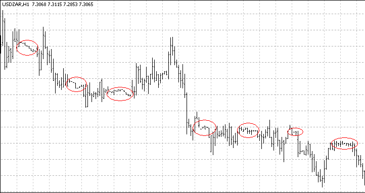
Moreover, the same effects are observed on popular currency pairs. This attracts interest to a more detailed examination of volumes and volatility behavior. It is clear that for a better understanding of intraday volatility fluctuations, crucially important is the behavior of volumes, i.e. ticks in a bar. But the volume itself is an accidental value, so we need to refer to the historical average. Such reference may appear not quite legal, if statistical "raw material" behaves in a "wrong" way.
For checking these hypotheses let us write a simple indicator - ExpectedVolume, which will find a historical average amount of ticks per hour, histSteps steps earlier, each step is span days long. Typical value of these parameters is accordingly 100 and 1. The testing is conducted on the timeframe H1, on other intraday timeframes parameters should be changed. Here is the indicator code:
//+------------------------------------------------------------------+
//|                                             Expected Volumes.mq4 |
//|                                     Copyright © 2007, Amir Aliev |
//|                                       http://finmat.blogspot.com/ |
//+------------------------------------------------------------------+
#property  copyright "Copyright © 2007, Amir Aliev"
#property  link      "http://finmat.blogspot.com/"
//----
#property indicator_separate_window
#property indicator_buffers 1
#property indicator_color1 Blue
//---- input parameters
extern int hist_steps = 100;      // Number of observations
extern int span = 1;              // Days to step back each time
//---- buffers
double ExtMapBuffer1[];
int sum;
//+------------------------------------------------------------------+
//| Custom indicator initialization function                         |
//+------------------------------------------------------------------+
int init()
  {
   string short_name;
//---- indicators
   SetIndexStyle(0, DRAW_HISTOGRAM);
   SetIndexBuffer(0,ExtMapBuffer1);
//----
   short_name = "Expected volumes(" + hist_steps + ")";
   IndicatorShortName(short_name);
   SetIndexLabel(0, short_name);
   return(0);
  }
//+------------------------------------------------------------------+
//| Custom indicator deinitialization function                       |
//+------------------------------------------------------------------+
int deinit()
  {
//----
   return(0);
  }
//+------------------------------------------------------------------+
//| Custom indicator iteration function                              |
//+------------------------------------------------------------------+
int start()
  {
   int counted_bars = IndicatorCounted();
   int rest = Bars - counted_bars;
   int j, k, u;
//----
   while(rest >= 0)
     {
      if(Bars - rest < span * 23 * hist_steps)
        {
         ExtMapBuffer1[rest] = 0;
         rest--;
         continue;
        }
      sum = 0;
      j = 0;
      k = 0;
      u = 0;
      while(j < hist_steps && k < Bars)
        {
         if(TimeHour(Time[rest+k]) == TimeHour(Time[rest]))
           {
            u++;
            if(u == span)
              {
               u = 0;
               j++;
               sum += Volume[rest + k];
              }
            k += 23;
           }
         k++;
        }
      ExtMapBuffer1[rest] = sum / hist_steps;
      rest--;
     }
//----
   return(0);
  }
//+------------------------------------------------------------------+
Still for checking the statistical homogeneity the observations should be independent, for examples divided into weekdays. For this purpose assign span=5. Get the following:
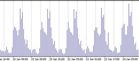
Neighboring humps are almost identical. It means the volatility, valued in ticks per hour, is statistically homogeneous. The structure of this volatility is clear from the pictures below (the left one - EURUSD, the right one - USDJPY):
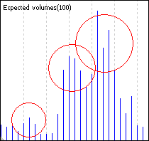
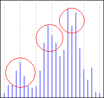
They vividly show three peaks of trading sessions' activity - Asian, European and American. It should be noted, that the division exactly into these trading sessions is not conventional - sometimes other sessions are singled out. Well, we can notice some peculiarities, for example the activity character during American session (is repeated on both charts).
Change of Indicators
When changing indicators it is very important to understand, how exactly time is included into them. For simple indicators, like Moving Average, this is quite easy, while it is quite difficult to change, for example, an Alligator.
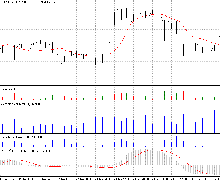
Finally it would be more rational to introduce an "operational" timeframe. But now let us try to change some simple indicators. The most primitive of them is corrected volumes - actual volumes are divided by expected ones. So the deviation into this or that side from 1 of this indicator reflects the increased/decreased activity on the market. The code is very simple. It is included into a file, attached to this article.
The next example is Average. Actually, we need just to weight the bar characteristic, upon which the average is built (for example, open), by the amount of ticks inside the bar. The final number is not equal exactly to the sum of price values on all ticks. For a more precise estimation we need to take not 'open', but a weighted average on a bar. The indicator is brute-force built, and that is why its calculation requires substantial and actually unnecessary computation costs. That is why one more parameter is added - the amount of bars from the past, which an indicator will draw, is by default equal to 500. Moreover the period of the average is set not in bars, but in the amount of ticks. Here is a code:
//+------------------------------------------------------------------+
//|                                                Corrected SMA.mq4 |
//|                                      Copyright © 2007, Amir Aliev |
//|                                    http://finmat.blogspot.com/   |
//+------------------------------------------------------------------+
#property copyright "Copyright © 2007, Amir Aliev"
#property link      "http://finmat.blogspot.com/"
//----
#property indicator_chart_window
#property indicator_color1 Red
//---- input parameters
extern int MA_Ticks = 10000;
extern int MA_Shift = 0;
extern int MA_Start = 500;
//---- indicator buffers
double ExtMapBuffer[];
double ExpVolBuffer[];
//+------------------------------------------------------------------+
//| Custom indicator initialization function                         |
//+------------------------------------------------------------------+
int init()
  {
//----
   SetIndexStyle(0, DRAW_LINE);
   SetIndexShift(0, MA_Shift);
   IndicatorBuffers(2);
//---- indicator buffers mapping
   SetIndexBuffer(0, ExtMapBuffer);
   SetIndexBuffer(1, ExpVolBuffer);
   SetIndexDrawBegin(0, 0);
//---- initialization done
   return(0);
  }
//+------------------------------------------------------------------+
//| Custom indicator iteration function                              |
//+------------------------------------------------------------------+
int start()
  {
   int counted_bars = IndicatorCounted();
   int rest  = Bars - counted_bars;
   int restt = Bars - counted_bars;
   double sum;
   int ts;
   int evol;
   int volsum;
   int j;
//----
   while(restt >= 0)
     {
       volsum = 0;
       for(int k = 0; k < 30; k++)
           volsum += iVolume(NULL, 0, restt + k*24);
       ExpVolBuffer[restt] = volsum / 30;
       restt--;
     }
//----
   while(ExpVolBuffer[rest] == 0 && rest >= 0)
       rest--;
   rest -= MA_Ticks / 200;
   if(rest > MA_Start)
       rest = MA_Start;
//----
   while(rest >= 0)
     {
       sum = 0;
       ts = 0;
       j = rest;
       while(ts < MA_Ticks)
         {
           evol = ExpVolBuffer[j];
           Print("Evol = ", evol);
           if(ts + evol < MA_Ticks)
             {
               sum += evol * Open[j];
               ts += evol;
             }
           else
             {
               sum += (MA_Ticks - ts) * Open[j];
               ts = MA_Ticks;
             }
           j++;
         }
       ExtMapBuffer[rest] = sum / MA_Ticks;
       rest--;
     }
//----
   return(0);
  }
//+------------------------------------------------------------------+
After the simple indicators are written, it will not be a problem to change more complex ones. Thus, for example in MACD code a adjusted moving average should be used instead a simple one. The corresponding code is also given in the attachment.
It should be noted, that for a quick calculation of the adjusted average, the empirical average of ticks per hour should be calculated once, and not on the fly of course, in order to avoid recalculations. It was omitted here, but if we conduct a full-scale testing/optimization on a history, the productivity comes to the front. Besides, there are admirers of another approach to building an adjusted upon volumes average, which should be discussed separately.
It would seem senseless to average volumes of previous periods: available volumes used as coefficients are enough in the average calculation. Here is an example of such a code. Still, it should be noted, that on technical grounds such an average is best of all used on small timeframes, like M1-M5.
//+------------------------------------------------------------------+
//|                                             Corrected SMA II.mq4 |
//|                                     Copyright © 2007, Amir Aliev |
//|                                       http://finmat.blogspot.com/ |
//+------------------------------------------------------------------+
#property copyright "Copyright © 2007, Amir Aliev"
#property link      "http://finmat.blogspot.com/"

#property indicator_chart_window
#property indicator_color1 Red
//---- input parameters
extern int MA_Ticks = 1000;
//---- indicator buffers
double sum = 0;
int ticks = 0;
bool collected = false;
bool started = false;
int fbar = 0;
double ExtMapBuffer[];
int oldRange = 0;
int lbarVol = 0;
//+------------------------------------------------------------------+
//| Custom indicator initialization function                         |
//+------------------------------------------------------------------+
int init()
  {
//----
   SetIndexStyle(0, DRAW_LINE);
//---- indicator buffers mapping
   SetIndexBuffer(0, ExtMapBuffer);
//---- initialization done
   return(0);
  }
//+------------------------------------------------------------------+
//| Custom indicator iteration function                              |
//+------------------------------------------------------------------+
int start()
  {
   int rest = Bars - IndicatorCounted();
   if(! rest)
       return (0);
   Print("Ticks = ", ticks);
   Print("Rest = ", rest);
   Print("fbar = ", fbar);
   rest--;
   fbar += rest;
   while(!collected && (rest >= 0))
     {
      if(ticks + Volume[rest] < MA_Ticks)
        {
         ticks += Volume[rest];
         sum += Volume[rest] * Open[rest];
         if(!started)
           {
            fbar = rest;
            started = true;
           }
         rest--;
         continue;
        }
      collected = true;
     }
   if(! collected)
       return (0);

   ticks += (Volume[rest] - lbarVol);
   sum += (Volume[rest] - lbarVol) * Open[rest];
   lbarVol = Volume[rest];
   while(ticks > MA_Ticks)
     {
       Print("fbar-- because bar ticks reaches 1000");
       ticks -= Volume[fbar];
       sum -= Volume[fbar] * Open[fbar];
       fbar--;
     }
   ExtMapBuffer[rest] = sum / ticks;
   rest--;
   while(rest >= 0)
     {
      ticks += Volume[rest];
      sum += Volume[rest] * Open[rest];
      lbarVol = Volume[rest];
      while(ticks > MA_Ticks)
        {
         Print("fbar-- because of new bar ");
         ticks -= Volume[fbar];
         sum -= Volume[fbar] * Open[fbar];
         fbar--;
        }
      ExtMapBuffer[rest] = sum / ticks;
      rest--;
     }
//----
   return(0);
  }
//+------------------------------------------------------------------+
However, the author thinks, though using this indicator can be helpful in some cases, generally it has the meaning, different from the one described in this article. The idea to take into account price values, for which there was a large "struggle" in the market, is quite artificial, also because small value deviations can be caused by technical reasons, and not market ones. Besides, it seems not reasonable to take into account the volatility change (and this is what we are talking about).
Each presented indicator can be amended allowing for specific tasks, for example changing an average for accounting the sum of values inside a bar or changing parameters of an average calculation. Remember, we have calculated through "open", which visually creates a feeling of a delay - the conception of time transformation, devolatilization allows a wide interpretation, including the ones, not discussed in this article, like seasonal volatility.
Conclusion
It should be noted, that while the price average is a quite unstable and hard-to-forecast value, the volatility, i.e. the second moment of increment, from the point of view of statistics is rather more "pleasant" and has a lot of well-known characteristics, like cluster properties, lever effect in stock markets and others.
That is why the conception of the operational time itself is quite useful and natural from the point of view of the technical analysis. Of course the fact that for example some key news about the economy state is released at a certain time, breaks the homogeneity quite seriously and is hardly "treated". But in the majority of cases using time transformation allows getting more stable results and increasing the profitability of a trading strategy.