Econometrics EURUSD One-Step-Ahead Forecast
СанСаныч Фоменко | 23 April, 2012
Introduction
The article focuses on one-step-ahead forecasting for EURUSD using EViews software and a further evaluation of forecasting results by means of the program in EViews and an Expert Advisor developed in MQL4. It is built up on the article "Analyzing the Indicators Statistical Parameters" whose propositions will be used without any additional clarifications.
1. Building a Model
The previous article ended with the analysis of the following regression equation:
EURUSD = C(1)*EURUSD_HP(1) + C(2)*D(EURUSD_HP(1)) + C(3)*D(EURUSD_HP(2))
This equation was a result of implementation of the gradual decomposition of the initial Close price quotes. The idea behind it is based on separation of a deterministic component from the initial quotes and a further analysis of the resulting residual.
Let us start building a model for EURUSD H1 on the bars over a period of one week from September 12, 2011 to September 17, 2011.
1.1. Analysis of the initial EURUSD quotes
We start off with the analysis of the initial EURUSD series in order to plan the next step.
First, let us create a file containing quotes for further analysis in EViews. For this purpose, I use an indicator superimposed on a relevant chart to generate a required file with quotes.
The script of the indicator is shown below and in my opinion needs no comment.
//+------------------------------------------------------------------+
//|                                                   Kotir_Out.mq4  |
//|   Quotes output indicator for EViews                             |
//|   Version of 29.08.2011                                          |
//+------------------------------------------------------------------+
//--- indicator in the main window
#property indicator_chart_window
//--- number of visible indicator buffers
#property indicator_buffers            1
//--- setting the indicator color
#property indicator_color1             Red      // Forecast
//--- setting the line width
#property indicator_width1             2
//--- external parameters
extern   int      Number_Bars=100;     // Number of bars
extern   string   DateTime_begin    =  "2011.01.01 00:00";
extern   string   DateTime_end      =  "2011.01.01 00:00";
//--- global variables
//--- declaring buffers
double   Quotes[];         // Quotes not visible
int      Quotes_handle;    // Pointer to Quotes file
int      i;                // Counter in cycle
//--- names of files for exchange with EViews
string   fileQuotes;       // Quotes file name
//+------------------------------------------------------------------+
//|Indicator initialization function                                 |
//+------------------------------------------------------------------+
int init()
  {
//--- number of indicator buffers
   IndicatorBuffers(1);
//--- setting the drawing parameters
   SetIndexStyle(0,DRAW_LINE,STYLE_SOLID,0);
   SetIndexDrawBegin(0,Number_Bars);

//--- binding the indicator number to the name
   SetIndexBuffer(0,Quotes);  // Index buffer

//--- initial buffer values
   SetIndexEmptyValue(0,0.0);
//--- indicator name
   IndicatorShortName("Forecast");
//--- generating names of files for exchange with EViews
   fileQuotes="kotir.txt";   // Quotes file name
   int       N_bars_begin   =  0;
   int       N_bars_end     =  0;

   datetime  var_DT_begin   =  0;
   datetime  var_DT_end     =  0;
   bool      exact          =  false;
//---
//--- creating quotes file for EViews operation
   Quotes_handle=FileOpen(fileQuotes,FILE_CSV|FILE_WRITE,',');
//--- abend exit
   if(Quotes_handle<1)
     {
      Print("Failed to create the file ",fileQuotes," Error #",GetLastError());
      return(0);
     }
   FileWrite(Quotes_handle,"DATE","kotir");  // Header
//---
//--- calculating the number of bars for export
   var_DT_begin =  StrToTime(DateTime_begin);
   var_DT_end   =  StrToTime(DateTime_end);

   if(var_DT_begin!=var_DT_end)
     {
      N_bars_begin=iBarShift(NULL,Period(),var_DT_begin,exact);
      N_bars_end=iBarShift(NULL,Period(),var_DT_end,exact);
      Number_Bars=N_bars_begin-N_bars_end;

      Print("Number_Bars = ",Number_Bars,
            ", N_bars_end = ",N_bars_end,
            ", N_bars_begin = ",N_bars_begin);

      for(i=N_bars_begin; i>=N_bars_end; i--)
        {
         FileWrite(Quotes_handle,
                   TimeToStr(iTime(Symbol(),Period(),i)),
                   iOpen(Symbol(),Period(),i));
        }
     }
   else
     {
      for(i=Number_Bars-1; i>=0; i--)
        {
         FileWrite(Quotes_handle,
                   TimeToStr(iTime(Symbol(),Period(),i)),
                   iOpen(Symbol(),Period(),i));
        }
     }
// --- writing quotes
   FileWrite(Quotes_handle, "Forecast ", 0);   // Forecast area
   FileClose(Quotes_handle);                  // Close quotes file
   Comment("Created quotes file with the number of bars =",Number_Bars+1);
//--- end of Init() section
   return(0);
  }
//+------------------------------------------------------------------+
//| Indicator start function                                         |
//+------------------------------------------------------------------+
int start()
  {
   return(0);
  }
//+------------------------------------------------------------------+
//| Custom indicator deinitialization function                       |
//+------------------------------------------------------------------+
int deinit()
  {
//--- remove the message from the display
   Comment("                                                     ");
//----
   return(0);
  }
//+------------------------------------------------------------------+
Having set the dates specified above, I obtained the quotes file consisting of 119 lines, the last line being "Forecast,0" – this is where the future forecast will be. Bear in mind that I am using Open prices. Also note that the quotes in the file are arranged in the order opposite to that of MQL4, i.e. as in programming languages.
The indicator obviously generates the file quotes.txt in the terminal folder \expert\files\. The Expert Advisor which is going to be reviewed below will take the quotes file from the specified folder when operating in DEMO or REAL modes; however when used in testing mode, this file shall be located in the \tester\files\ folder so I am manually placing quotes.txt in the \tester\files\ folder of the terminal.
Here is the chart:
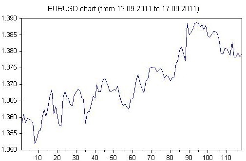
Fig. 1. EURUSD H1 quotes chart
We can observe either one or numerous trends but our goal is to predict the future stability of the trading system. Therefore we will perform an analysis for stationarity of the initial EURUSD H1 quotes.
Let us calculate the descriptive statistics:
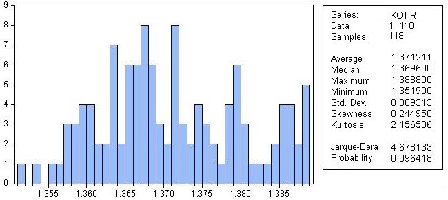
Fig. 2. Descriptive statistics
The descriptive statistics suggests that:
- There is a skew to the right (it should be 0 whereas we have 0.244950);
- The probability of our initial quotes to be normally distributed is 9.64%.
Visually, the histogram has certainly nothing to do with the normal distribution but the probability of 9.64% gives rise to certain illusions.
Let us demonstrate it compared to the theory:
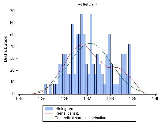
Fig. 3. EURUSD histogram as compared to theoretical normal distribution curve
We can visually ascertain that the EURUSD_Рќ1 quotes are far from being normally distributed.
However, it is still early to draw a conclusion as we can see the trend suggesting the presence of a deterministic component in the quotes whereas the presence of such component can completely distort the statistical characteristics of the random variable (quotes).
Let us calculate autocorrelation function of the quotes.
It appears as follows:
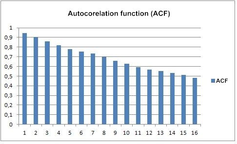
Fig. 4. Autocorrelation function of the EURUSD_H1 quotes
When plotting the chart, we have obtained a probability of the lack of correlation between the lags - it is nonzero for the first 16 lags. The chart and probability clearly suggest that there is correlation between the lags in EURUSD_H1, i.e. the quotes under consideration contain a deterministic component.
If the deterministic component is subtracted from the initial quotes, what statistical characteristics will the residual have?
For this purpose, we will apply a unit root test to see whether it is more prospective to work with the first difference (residual) of the initial quotes.
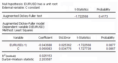
Table 1. Unit root test
The above test shows that:
- The probability that the initial quotes have a unit root (the first difference is normally distributed) is 41%;
- The DW (Durbin-Watson) statistic is just over 2.2 which also suggests that the first difference is normally distributed.
1.2. Smoothing
The Hodrick-Prescott filter will be used to separate out the deterministic component from the EURUSD quotes, by analogy with the previous article.
Number "10" in the series names denotes the lambda parameter in the Hodrick-Prescott filter. Based on the theory behind this tool, the lambda value is of great importance for the result which appears to be as follows:
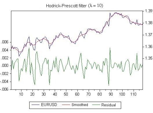
Fig. 5. The smoothing result using the Hodrick-Prescott filter
We will use the equation from the previous article which in the EViews notations appears as follows:
quotes = C(1) * HP(-1) + C(2) * D(HP(-1)) + C(3)*D(HP(-2))
i.e. in this equation, we take into account the deterministic component and noise by which we mean the difference between the initial quotes and its deterministic component.
Following the analysis of the current model of the initial quotes, we obtain the following regression equation parameters:
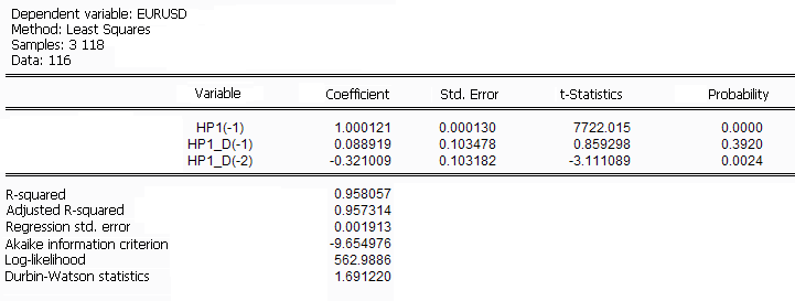
Table 2. Regression equation estimation
The 39% probability of the coefficient being zero if РќР 1_D(-1) is certainly extremely displeasing. We will leave everything as it is since the example we are going to provide is for demonstration purposes.
Having obtained the regression equation estimates (estimation of the equation coefficients) we can proceed to the one-step-ahead forecast.
The result is as follows:
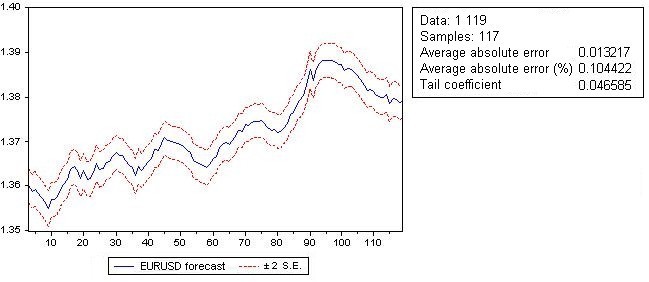
Fig. 6. EURUSD one-step-ahead forecast (as at 12 a.m. on Monday)
1.3. Estimating residuals from the regression equation
Let us perform a limited analysis of the residual from the regression equation. This residual was obtained by subtracting the values calculated using the regression equation from the initial EURUSD quotes.
Let me remind you that the characteristics of this residual will help us estimate the future stability of the trading system.
First, we will run a test for the analysis of correlations between the lags in the residual:
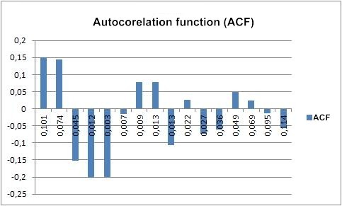
Fig. 7. Autocorrelation function of the residual
Unfortunately, the correlations between the lags are still there and their presence casts doubt on the statistical analysis.
The next test we are going to perform is the normality test of the residual.
The result appears as follows:
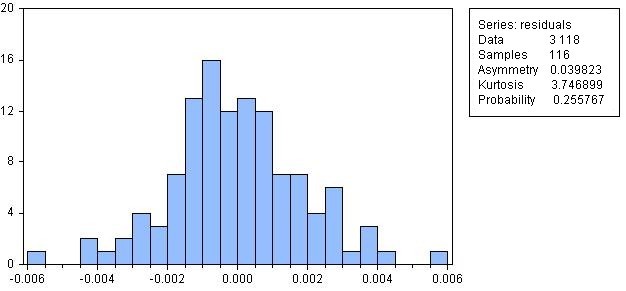
Fig. 8. Histogram of the residual from the regression equation
The probability of the residual to be normally distributed is 25.57% which is quite a big figure.
Let us perform tests for heteroscedasticity of the residual.
The results are as follows:
- The probability that GARCH-type heteroscedasticity is absent is 16.08%
- The probability that White's general heteroscedasticity is absent is 0.0066%
Since my aim is to demonstrate trading system development based on the forecast, I am going to continue calculations in order to obtain the characteristics that are of interest to traders - profit or loss.
2. Estimating Forecast Results
When trading, we are interested in profit rather than forecast error which should be taken as an auxiliary analysis tool for comparison of different models but not more than that.
To estimate the forecast results, a program in the EViews language was written. It compares actual incremental movements of the EURUSD quotes with the predicted ones. If these increments coincide, there is profit; if they don't, there is loss. Further, we calculate profit which represents the sum of all increments coinciding with the predicted increments, and the respective loss.
The profit to loss ratio is designated as a profit factor. We then calculate the ratio of profitable to unprofitable increments (profit to loss trades ratio). The number of consecutive loss trades and the ratio of loss in consecutive loss trades to profit (recovery factor) is also calculated.
The program in the EViews language for estimation of modeling results in terms of trading system consists of the main program and two subroutines.
The main (head) program is as follows:
'
' One-step-ahead forecasting program
' Version of 26.09.2011
'-----------------------------------------------
 include    sub_profit_factor
 include    sub_model_2
'
' 1. Create an EViews work file under the name МТ4
'
 %path   = "C:\Program Files\BCS Trade Station\tester\files"
 cd      %path

 if @fileexist("work.wf1") = 0  then
  wfcreate(wf  = work)  u 510
 else
  wfopen   work
 endif
'
' Reads quotes from files
 read(t = txt)   kotir.txt date $ kotir
'
' Number of observations in the series without NA
 !number   = @obs(kotir)
 smpl     1  !number  - 1


 genr  trend    = NA        ' Trend = kotir_f(i) - kotir(i-1)
 genr  kotir_d  = d(kotir)  ' One-step increment in the price movement  - d(kotir)
'

' Calculate the model
 call  sub_model_2
'
' Calculate the profit table
 call sub_profit_factor

' Generate a file of results
 genr result   = 0
'
' Fill in the results
 result(1)  = kotir_f(!number)    ' One-step-ahead forecast
 result(2)  = kotir_f_se(!number) ' One-step-ahead forecast error
 result(3)  = trend(!number - 1)  ' Direction of the forecast
'-----------------------------------------------
' Return the result to МТ4
'
 smpl      1  10
 write(t=txt,na=0,d=c,dates)  EViewsForecast.txt   result

'-----------------End of program --------------
 smpl      1  !number
 save       work
 close      @all
 exit
'
'-----------------------------------------------
It is assumed that the number of the main programs is equal to the number of subroutines containing models (see below); this is done for simplification of work.
The change in the model requires a change in two lines of the main program relating to the change in the name of the subroutine for the model.
The subroutine containing the model (regression equation):
subroutine  sub_model_2

  cd
  wfselect             work
  smpl          1    !number    -  1
' Smoothing the 1st level using НР filter quote with the first lambda
' and generating two files:
'      hp1     -  smoothed file
'      p1_d    -   file of the residual
  hpf(lambda    =  10)   kotir hp1   @hp1_d
'
'  4. Estimating regression eq02 that uses the following series:
'        hp1
'        hp1_d
  equation eq1.ls   kotir   hp1(-1)   hp1_d(-1) hp1_d(-2)


'
'  Extending the sample to include the forecast area
  smpl              1 !number
'
'  Performing a one-step-ahead forecast and generating output series:
'    kotir_f     -  forecast
'    kotir_f_se  -  forecast error
  fit(p)            kotir_f   kotir_f_se

  save              work

endsub
The number of subroutines shall be equal to the number of models.
For another model, the name of the subroutine and, naturally, the names in the main program shall be changed.
Subroutine that calculates profit/loss parameters for the model:
' Subroutine for estimation of the forecast results
' Version of 27.09.2011
' ----------------------------------------------------------------------------
' Comparing the forecast increment with the quote increment,
' the program calculates:
'  profit factor with regard to increments;
'   profitability of the equation in the number of observations
'  recovery factor as a ratio of profit in pips to maximal drawdown
' ----------------------------------------------------------------------------
subroutine sub_profit_factor

' Local variables
   !profit = 0          ' Accumulated profit
   !lost = 0            ' Accumulated loss
   !profit_factor = 0   ' Profit factor
   !i = 1               ' Work index
   !n_profit = 0        ' Number of profit trades
   !n_lost = 0          ' Number of loss trades
   !n_p_l = 0           '
   !pr = 0              '  Absence of consecutive losses
   !prosadka = 0        ' Drawdown - accumulation of consecutive losses
   !tek_prosadka = 0    ' Current drawdown
   !tek_pr = 0          '  Current number of loss trades

 cd
 wfselect       work
 smpl        1   !number

' Calculate the trend on each bar
 for  !i  =  1  to  !number - 1
  trend(!i) = kotir_f(!i + 1) - kotir(!i)
 next

'  Calculate profit if the forecast has been reached
 for  !i      =  1   to  !number - 1
  if  trend(!i) * kotir_d(!i) > 0   then    ' Does the trend coincide with increment? - Yes
   !profit   = !profit + @abs(kotir_d(!i))  '  Profit accumulation
   !n_profit = !n_profit +1                 '  Profit trades accumulation
   !tek_pr   = 0                            '  Resetting the current consecutive losses at zero
   !tek_prosadka  =   0                     ' Resetting the current drawdown at zero
  endif
  if  trend(!i) * kotir_d(!i) <  0   then   ' Does the trend coincide with increment? - No
   !lost   = !lost + @abs(kotir_d(!i))      ' Loss accumulation
   !n_lost = !n_lost + 1                    ' Loss trades accumulation

   !tek_pr = !tek_pr + 1                              ' Increase the number of current loss trades
   !tek_prosadka = !tek_prosadka + @abs(kotir_d(!i))  ' Increase the current drawdown
  endif

  '  Select the maximum loss trades
  if  !tek_pr > !pr then
   !pr  = !tek_pr
  endif

  ' Select the maximal drawdown
  if  !tek_prosadka  > !prosadka  then
   !prosadka  = !tek_prosadka
  endif
 next

'   Blocking division by zero
 if !lost = 0 then                 ' No loss trades
  !profit_factor = 1000
 else
  !profit_factor = !profit / !lost  ' Profit factor
 endif

 if !n_lost = 0  then
  !n_p_l = !number      '  if loss trades are zero,
                        '  profit trades are equal to the number of observations
 else
  !n_p_l =  !n_profit / !n_lost
 endif

 if !prosadka = 0  then
  !factor_reset = 1000
 else
  !factor_reset = !profit / !prosadka
 endif

'  Create a table of results if it does not exist
 if @isobject("tab_profit") = 0    then
  table(3,12)    tab_profit
  tab_profit.title  One-step-ahead forecast after the end of sample with profitability beyond the sample

' Make the table heading
  tab_profit.setfillcolor(1) yellow
  tab_profit.setfillcolor(2) yellow

' Set the column characteristics
' 1st column
  setcolwidth(tab_profit,1,15)
  tab_profit(1,1)   = "Sample"
  tab_profit(2,1)   = "beginning"

' 2nd column
  setcolwidth(tab_profit,2,15)
  tab_profit(1,2)   = "Sample"
  tab_profit(2,2)   = "end"

' 3rd column
  setcolwidth(tab_profit,3,7)
   tab_profit(1,3)   = "Fact as of"
  tab_profit(2,3)   = "end "

' 4th column
  setcolwidth(tab_profit,4,7)
  tab_profit(1,4)   = "One-step"
  tab_profit(2,4)   = "forecast"

' 5th column
  setcolwidth(tab_profit,5,10)
  tab_profit(1,5)   = "Forecast"
  tab_profit(2,5)   = "error"

' 6th column
  setcolwidth(tab_profit,6,8)
  tab_profit(1,6)    =  "Profit of the"
  tab_profit(2,6)    =  "sample"

' 7th column
  setcolwidth(tab_profit,7,8)
  tab_profit(1,7)    =  "Loss of the"
  tab_profit(2,7)    =  "sample"

' 8th column
  setcolwidth(tab_profit,8,10)
  tab_profit(1,8)   = "Maximal"
  tab_profit(2,8)   = "drawdown"

' 9th column
  setcolwidth(tab_profit,9,8)
  tab_profit(1,9)   = "Amount of"
  tab_profit(2,9)    =  "loss"

' 10th column
  setcolwidth(tab_profit,10,7)
  tab_profit(1,10)    =  "P / F in"
  tab_profit(2,10)    =  "pips"

' 11th column
  setcolwidth(tab_profit,11,8)
  tab_profit(1,11)    =  "P / F in"
  tab_profit(2,11)    =  "observations"


' 12th column
  setcolwidth(tab_profit,12,8)
  tab_profit(1,12)   = "Recovery"
  tab_profit(2,12)   = "factor"
  tab_profit.setlines(R1C1:R2C12) +o +v
 endif

 tab_profit.insertrow(3) 1
 tab_profit.setlines(R3C1:R3C12) +a +v +i

' Set the table output format
 tab_profit.setformat(R3C1:R3C1)   c.16
 tab_profit.setformat(R3C2:R3C2)   c.16
 tab_profit.setformat(R3C3:R3C3)   f.4
 tab_profit.setformat(R3C4:R3C4)   f.4
 tab_profit.setformat(R3C5:R3C5)   f.4
 tab_profit.setformat(R3C6:R3C6)   f.4
 tab_profit.setformat(R3C7:R3C7)   f.4
 tab_profit.setformat(R3C8:R3C8)   f.4
 tab_profit.setformat(R3C9:R3C9)   f.0
 tab_profit.setformat(R3C10:R3C10) f.2
 tab_profit.setformat(R3C11:R3C11)  f.2
 tab_profit.setformat(R3C12:R3C12) f.2

' Fill the table with the results
 tab_profit(3 ,1) = date(1)
 tab_profit(3 ,2) = date(!number - 1)
 tab_profit(3 ,3) = kotir(!number - 1)
 tab_profit(3 ,4) = kotir_f(!number - 1)
 tab_profit(3 ,5) = kotir_f_se(!number - 1)

 tab_profit(3 ,6) =  !profit
 tab_profit(3 ,7) =  !lost
 tab_profit(3 ,8) = !prosadka
 tab_profit(3 ,9) = !pr
 tab_profit(3,10) =  !profit_factor
 tab_profit(3,11) = !n_p_l
 tab_profit(3,12) = !factor_reset


' Save the table in the work file
 save        work
 show        tab_profit

endsub
The results of the above simple programs in EViews for our equation are as follows:

Table 3. Profitability estimation results in EViews
Until now, the EURUSD_H1 quotes have been analyzed using EViews tools.
However, it appears to be very tempting to apply the forecast results in an Expert Advisor of the MetaTrader 4 terminal.
Let us now consider the exchange of data between EViews and MetaTrader 4 and then once again analyze the results using an Expert Advisor in MetaTrader 4.
3. Data Exchange Between EViews and MetaTrader 4
Exchange of data between EViews and MetaTrader 4 in this article is implemented using .txt files.
The exchange algorithm appears to be as follows:
-
MetaTrader 4 Expert Advisor:
- Generates the quotes file;
- Starts EViews.
-
EViews:
- Starts operating in response to a command from the Expert Advisor;
- Runs a forecast calculation program for the quotes file quotes.txt obtained from the Expert Advisor;
- Saves the forecast results into the EViewsForecast.txt file.
-
MetaTrader 4 Expert Advisor:
- Upon completion of generation of the results in EViews, reads the forecast file;
- Decides on entering or exiting a position.
A few words about location of the files.
Files of the MetaTrader 4 terminal are placed in their standard folders: an Expert Advisor in the \expert folder and indicator (that is not required for testing) in the \expert\indicators folder. All of those are located in the terminal directory. The Expert Advisor is installed together with other Expert Advisors.
Files for exchange between the Expert Advisor and EViews are located in \expert\files during operation of the Expert Advisor and in the \tester\files folder when testing the Expert Advisor.
The file sent by the Expert Advisor to EViews is named quotes.txt regardless of the selected symbol and time frame. Therefore the Expert Advisor can be attached to any symbol while the forecast step shall be specified in the parameters of the Expert Advisor at its start.
EViews returns the file named EVIEWSFORECAST.txt. The EViews work file worf.wf1 is placed in the terminal directory.
Directories specified in the EViews programs that are attached to the article will most likely not match the directories you have available on your computers. I installed these programs in the disc root folder. In EViews, you will have to get a handle on the default directory or specify your own directories (I did not use the default directories utilized by EViews itself).
4. MQL4 Expert Advisor
The Expert Advisor operation algorithm is simplified to the maximum:
- The Expert Advisor is attached to M1 time frame of any symbol;
- A forecast step in minutes is specified in the parameters of the Expert Advisor. The default forecast step is 60 minutes (Рќ1). By attaching the Expert Advisor to M1, you get an opportunity to better visualize the testing results as the testing chart can be compressed when switching to a longer time frame;
- For the purposes of forecasting in EViews, the Expert Advisor generates the quotes.txt file with the number of bars (observations) as specified in the parameters of the Expert Advisor;
- If the forecast is greater than the current price, a long position opens;
- If the forecast is less than the current price, a short position opens;
- The Expert Advisor opens no more than one position (without adding to a position);
- Regardless of the forecast, it closes the preceding position and opens the new one. The algorithm for the opening of positions coincides with the algorithm for calculating profit/loss in the program in EViews;
- The volume of the position to be opened is 0.1 lot;
- Stop loss and take profit orders are not used (they are set at 100 pips although the Expert Advisor has a code for placing stops at forecast error intervals);
- A chart is drawn showing the forecast value and two lines at one standard forecast error interval. When viewing the chart from the tester on shorter time frames than the one to which the Expert Advisor was attached, bear in mind that the forecast line is shifted back, i.e. the forecast drawn is the forecast at which the current price should arrive at the end of the period.
The Expert Advisor is attached to M1 time frame while in the tester, the chart is better viewed on M5.
The source code of the MQL4 Expert Advisor for trading EURUSD is not provided in this article due to its volume (around 600 lines). It can be found in EvewsMT4.mq4 in the EViews_MetaTrader_4.zip archive attached to the article.
5. Expert Advisor Testing Results
Run the Expert Advisor in the tester on M1 time frame.
The input parameters are shown below.
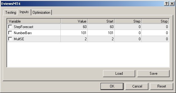
Fig. 9. Input parameters of the Expert Advisor
A fragment of the testing chart is demonstrated below:
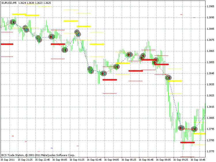
Fig. 10. Testing of the Expert Advisor in the visualization mode
The results of testing the Expert Advisor that uses one-hour (step) ahead forecasts are shown below.
Strategy Tester Report
EvewsMT4
Real (Build 406)
| Symbol | EURUSD (Euro vs US Dollar) | ||||
| Time Frame | 1 Minute (M1) 2011.09.12 00:00 - 2011.09.16 21:59 (2011.09.12 - 2011.09.17) | ||||
| Model | Every tick (the most accurate mode based on the shortest available time frames) | ||||
| Parameters | StepForecast=60; NumberBars=101; MultSE=2; | ||||
| Bars in the history | 7948 | Ticks modeled | 79777 | Modeling quality | 25.00% |
| Mismatched chart errors | 0 | ||||
| Initial deposit | 10000.00 | ||||
| Net profit | -202.10 | Gross profit | 940.72 | Gross loss | -1142.82 |
| Profit factor | 0.82 | Expected payoff | -1.73 | ||
| Absolute drawdown | 326.15 | Maximal drawdown | 456.15 (4.50%) | Relative drawdown | 4.50% (456.15) |
| Total trades | 117 | Short positions (won %) | 58 (51.72%) | Long positions (won %) | 59 (45.76%) |
| Profit trades (% of total) | 57 (48.72%) | Loss trades (% of total) | 60 (51.28%) | ||
| Largest | profit trade | 100.00 | loss trade | -79.00 | |
| Average | profit trade | 16.50 | loss trade | -19.05 | |
| Maximum | consecutive wins (profit in money) | 6 (105.00) | consecutive losses (loss in money) | 8 (-162.00) | |
| Maximal | consecutive profit (count) | 166.00 (5) | consecutive loss (count) | -162.00 (8) | |
| Average | consecutive wins | 2 | consecutive losses | 2
| |

| No. | Time | Type | Order | Volume | Price | S / L | T / P | Profit | Balance |
| 1 | 2011.09.12 01:00 | sell | 1 | 0.10 | 1.3609 | 1.3711 | 1.3509 | ||
| 2 | 2011.09.12 02:00 | close | 1 | 0.10 | 1.3584 | 1.3711 | 1.3509 | 25.00 | 10025.00 |
Fig. 11. Expert Advisor Testing Results
The results are better than those obtained in EViews.
Note that calculation of results in EViews and the tester is different in terms of input data. EViews uses 118 bars and calculates the forecast starting from the 3 bar on the left as the one-step-ahead forecast is gradually moving towards the end of the time period increasing the number of bars used in estimation of the regression equation.
The Expert Advisor shifts the window of 118 bars and calculates the forecast on bar 119, i.e. the regression equation is always estimated on 118 bars since EViews expands the window within the sample and the Expert Advisor shifts the window of fixed width.
The Expert Advisor helps us produce an extended model estimation table. While the table above consisted of a single line, it now contains 117 lines - for every date for which the forecast was produced.
The table is as follows:
| Beginning of the sample | End of the sample | Fact as of end | One-step forecast | Forecast error | Profit of the sample | Loss of the sample | Maximal drawdown | Amount of losses | P/F in pips | P/F in observations | Recovery factor |
|---|---|---|---|---|---|---|---|---|---|---|---|
| 12.09.2011 0:00 | 16.09.2011 21:00 | 1,3791 | 1,3788 | 0,0019 | 0,0581 | 0,1531 | 0,0245 | 7 | 0,38 | 0,67 | 2,37 |
| 12.09.2011 0:00 | 16.09.2011 21:00 | 1,3791 | 1,3788 | 0,0019 | 0,0581 | 0,1531 | 0,0245 | 7 | 0,38 | 0,67 | 2,37 |
| 09.09.2011 21:00 | 16.09.2011 20:00 | 1,3784 | 1,3793 | 0,0019 | 0,0569 | 0,1619 | 0,0245 | 7 | 0,35 | 0,64 | 2,32 |
| 09.09.2011 20:00 | 16.09.2011 19:00 | 1,3794 | 1,3796 | 0,002 | 0,0596 | 0,1609 | 0,0245 | 7 | 0,37 | 0,67 | 2,43 |
| 09.09.2011 19:00 | 16.09.2011 18:00 | 1,3783 | 1,3782 | 0,0021 | 0,0642 | 0,1554 | 0,0245 | 7 | 0,41 | 0,69 | 2,62 |
| 09.09.2011 18:00 | 16.09.2011 17:00 | 1,3783 | 1,3806 | 0,002 | 0,0616 | 0,1606 | 0,0245 | 7 | 0,38 | 0,68 | 2,51 |
| 09.09.2011 17:00 | 16.09.2011 16:00 | 1,3829 | 1,3806 | 0,002 | 0,0642 | 0,1586 | 0,0245 | 7 | 0,4 | 0,71 | 2,62 |
| 09.09.2011 16:00 | 16.09.2011 15:00 | 1,3788 | 1,3793 | 0,002 | 0,0626 | 0,1565 | 0,0245 | 7 | 0,4 | 0,71 | 2,56 |
| 09.09.2011 15:00 | 16.09.2011 14:00 | 1,3798 | 1,38 | 0,0021 | 0,063 | 0,1633 | 0,0245 | 7 | 0,39 | 0,73 | 2,57 |
| 09.09.2011 14:00 | 16.09.2011 13:00 | 1,3808 | 1,381 | 0,0022 | 0,062 | 0,1656 | 0,0318 | 9 | 0,37 | 0,71 | 1,95 |
| 09.09.2011 13:00 | 16.09.2011 12:00 | 1,3809 | 1,3813 | 0,0021 | 0,0602 | 0,1679 | 0,0318 | 9 | 0,36 | 0,66 | 1,89 |
| 09.09.2011 12:00 | 16.09.2011 11:00 | 1,3792 | 1,3808 | 0,0021 | 0,0666 | 0,1613 | 0,0245 | 7 | 0,41 | 0,73 | 2,72 |
| 09.09.2011 11:00 | 16.09.2011 10:00 | 1,3795 | 1,3826 | 0,0021 | 0,0666 | 0,167 | 0,0245 | 7 | 0,4 | 0,73 | 2,72 |
| 09.09.2011 10:00 | 16.09.2011 9:00 | 1,3838 | 1,3847 | 0,0022 | 0,0652 | 0,1668 | 0,0318 | 9 | 0,39 | 0,71 | 2,05 |
| 09.09.2011 9:00 | 16.09.2011 8:00 | 1,3856 | 1,3854 | 0,0022 | 0,0675 | 0,165 | 0,0318 | 9 | 0,41 | 0,73 | 2,12 |
| 09.09.2011 8:00 | 16.09.2011 7:00 | 1,386 | 1,3856 | 0,0022 | 0,0671 | 0,1652 | 0,0318 | 9 | 0,41 | 0,71 | 2,11 |
| 09.09.2011 7:00 | 16.09.2011 6:00 | 1,3861 | 1,3857 | 0,0022 | 0,067 | 0,1663 | 0,0318 | 9 | 0,4 | 0,68 | 2,11 |
| 09.09.2011 6:00 | 16.09.2011 5:00 | 1,3852 | 1,3855 | 0,0022 | 0,0655 | 0,1681 | 0,0318 | 9 | 0,39 | 0,63 | 2,06 |
| 09.09.2011 5:00 | 16.09.2011 4:00 | 1,3844 | 1,3851 | 0,0022 | 0,0662 | 0,1674 | 0,0318 | 9 | 0,4 | 0,66 | 2,08 |
| 09.09.2011 4:00 | 16.09.2011 3:00 | 1,3848 | 1,3869 | 0,0022 | 0,0654 | 0,1683 | 0,0318 | 9 | 0,39 | 0,68 | 2,06 |
| 09.09.2011 3:00 | 16.09.2011 2:00 | 1,3879 | 1,3875 | 0,0022 | 0,0694 | 0,1624 | 0,0318 | 9 | 0,43 | 0,73 | 2,18 |
| 09.09.2011 2:00 | 16.09.2011 1:00 | 1,3865 | 1,3879 | 0,0022 | 0,0698 | 0,1634 | 0,0318 | 9 | 0,43 | 0,71 | 2,19 |
| 09.09.2011 1:00 | 16.09.2011 0:00 | 1,3881 | 1,3883 | 0,0022 | 0,0726 | 0,1604 | 0,0245 | 7 | 0,45 | 0,76 | 2,96 |
| 09.09.2011 0:00 | 15.09.2011 23:00 | 1,3876 | 1,3882 | 0,0022 | 0,0721 | 0,162 | 0,0245 | 7 | 0,45 | 0,73 | 2,94 |
| 08.09.2011 23:00 | 15.09.2011 22:00 | 1,3885 | 1,3884 | 0,0022 | 0,0718 | 0,1614 | 0,0245 | 7 | 0,44 | 0,72 | 2,93 |
| 08.09.2011 22:00 | 15.09.2011 21:00 | 1,3888 | 1,3883 | 0,0022 | 0,0737 | 0,1597 | 0,0245 | 7 | 0,46 | 0,77 | 3,01 |
| 08.09.2011 21:00 | 15.09.2011 20:00 | 1,3885 | 1,3874 | 0,0022 | 0,0729 | 0,1604 | 0,0318 | 9 | 0,45 | 0,74 | 2,29 |
| 08.09.2011 20:00 | 15.09.2011 19:00 | 1,3867 | 1,386 | 0,0022 | 0,0721 | 0,1604 | 0,0318 | 9 | 0,45 | 0,74 | 2,27 |
| 08.09.2011 19:00 | 15.09.2011 18:00 | 1,3856 | 1,3834 | 0,0022 | 0,0721 | 0,1628 | 0,0318 | 9 | 0,44 | 0,72 | 2,27 |
| 08.09.2011 18:00 | 15.09.2011 17:00 | 1,385 | 1,3861 | 0,0023 | 0,0702 | 0,1651 | 0,0318 | 9 | 0,43 | 0,72 | 2,21 |
| 08.09.2011 17:00 | 15.09.2011 16:00 | 1,3885 | 1,3824 | 0,0023 | 0,0739 | 0,1638 | 0,0245 | 7 | 0,45 | 0,72 | 3,02 |
| 08.09.2011 16:00 | 15.09.2011 15:00 | 1,3773 | 1,3784 | 0,0021 | 0,0719 | 0,1556 | 0,0318 | 9 | 0,46 | 0,72 | 2,26 |
| 08.09.2011 15:00 | 15.09.2011 14:00 | 1,3795 | 1,3794 | 0,0021 | 0,0726 | 0,1537 | 0,0318 | 9 | 0,47 | 0,72 | 2,28 |
| 08.09.2011 14:00 | 15.09.2011 13:00 | 1,3814 | 1,3792 | 0,0021 | 0,0736 | 0,1564 | 0,0318 | 9 | 0,47 | 0,74 | 2,31 |
| 08.09.2011 13:00 | 15.09.2011 12:00 | 1,3802 | 1,3764 | 0,0021 | 0,0712 | 0,159 | 0,0318 | 9 | 0,45 | 0,74 | 2,24 |
| 08.09.2011 12:00 | 15.09.2011 11:00 | 1,3769 | 1,3753 | 0,0021 | 0,0719 | 0,1568 | 0,0318 | 9 | 0,46 | 0,72 | 2,26 |
| 08.09.2011 11:00 | 15.09.2011 10:00 | 1,3765 | 1,3732 | 0,0021 | 0,0721 | 0,1564 | 0,0318 | 9 | 0,46 | 0,74 | 2,27 |
| 08.09.2011 10:00 | 15.09.2011 9:00 | 1,3722 | 1,3718 | 0,0021 | 0,0716 | 0,1538 | 0,0318 | 9 | 0,47 | 0,72 | 2,25 |
| 08.09.2011 8:00 | 15.09.2011 7:00 | 1,371 | 1,3716 | 0,0021 | 0,0729 | 0,1542 | 0,0318 | 9 | 0,47 | 0,74 | 2,29 |
| 08.09.2011 8:00 | 15.09.2011 7:00 | 1,371 | 1,3716 | 0,0021 | 0,0729 | 0,1542 | 0,0318 | 9 | 0,47 | 0,74 | 2,29 |
| 08.09.2011 7:00 | 15.09.2011 6:00 | 1,3723 | 1,3727 | 0,0021 | 0,0716 | 0,1547 | 0,0318 | 9 | 0,46 | 0,72 | 2,25 |
| 08.09.2011 6:00 | 15.09.2011 5:00 | 1,3726 | 1,3725 | 0,0021 | 0,0711 | 0,1564 | 0,0318 | 9 | 0,45 | 0,69 | 2,24 |
| 08.09.2011 5:00 | 15.09.2011 4:00 | 1,3719 | 1,3731 | 0,0021 | 0,0711 | 0,1563 | 0,0318 | 9 | 0,45 | 0,69 | 2,24 |
| 08.09.2011 4:00 | 15.09.2011 3:00 | 1,374 | 1,3744 | 0,0021 | 0,0713 | 0,1547 | 0,0318 | 9 | 0,46 | 0,69 | 2,24 |
| 08.09.2011 3:00 | 15.09.2011 2:00 | 1,3748 | 1,3747 | 0,0021 | 0,0705 | 0,1547 | 0,0318 | 9 | 0,46 | 0,68 | 2,22 |
| 08.09.2011 2:00 | 15.09.2011 1:00 | 1,3743 | 1,3742 | 0,0021 | 0,0715 | 0,1544 | 0,0318 | 9 | 0,46 | 0,7 | 2,25 |
| 08.09.2011 1:00 | 15.09.2011 0:00 | 1,3738 | 1,3743 | 0,0021 | 0,0714 | 0,1544 | 0,0318 | 9 | 0,46 | 0,7 | 2,25 |
| 08.09.2011 0:00 | 14.09.2011 23:00 | 1,375 | 1,3743 | 0,0021 | 0,0724 | 0,1532 | 0,0318 | 9 | 0,47 | 0,73 | 2,28 |
| 07.09.2011 23:00 | 14.09.2011 22:00 | 1,375 | 1,3736 | 0,0021 | 0,0727 | 0,1532 | 0,0318 | 9 | 0,47 | 0,74 | 2,29 |
| 07.09.2011 22:00 | 14.09.2011 21:00 | 1,3751 | 1,3735 | 0,0021 | 0,0734 | 0,1532 | 0,0318 | 9 | 0,48 | 0,74 | 2,31 |
| 07.09.2011 21:00 | 14.09.2011 20:00 | 1,3748 | 1,3716 | 0,0021 | 0,0722 | 0,1555 | 0,0318 | 9 | 0,46 | 0,72 | 2,27 |
| 07.09.2011 20:00 | 14.09.2011 19:00 | 1,3714 | 1,3712 | 0,0021 | 0,0812 | 0,145 | 0,0189 | 6 | 0,56 | 0,74 | 4,3 |
| 07.09.2011 19:00 | 14.09.2011 18:00 | 1,371 | 1,3697 | 0,0021 | 0,0692 | 0,1577 | 0,0318 | 9 | 0,44 | 0,69 | 2,18 |
| 07.09.2011 18:00 | 14.09.2011 17:00 | 1,3673 | 1,369 | 0,0021 | 0,0695 | 0,154 | 0,0318 | 9 | 0,45 | 0,72 | 2,19 |
| 07.09.2011 17:00 | 14.09.2011 16:00 | 1,3687 | 1,3693 | 0,0021 | 0,0695 | 0,1548 | 0,0318 | 9 | 0,45 | 0,72 | 2,19 |
| 07.09.2011 16:00 | 14.09.2011 15:00 | 1,3704 | 1,3704 | 0,0021 | 0,066 | 0,1591 | 0,0318 | 11 | 0,41 | 0,69 | 2,08 |
| 07.09.2011 15:00 | 14.09.2011 14:00 | 1,373 | 1,37 | 0,002 | 0,066 | 0,1577 | 0,0318 | 10 | 0,42 | 0,69 | 2,08 |
| 07.09.2011 14:00 | 14.09.2011 13:00 | 1,3712 | 1,3681 | 0,002 | 0,066 | 0,1562 | 0,0318 | 9 | 0,42 | 0,69 | 2,08 |
| 07.09.2011 13:00 | 14.09.2011 12:00 | 1,3685 | 1,3653 | 0,002 | 0,0665 | 0,1534 | 0,0318 | 9 | 0,43 | 0,74 | 2,09 |
| 07.09.2011 12:00 | 14.09.2011 11:00 | 1,3655 | 1,3646 | 0,002 | 0,0673 | 0,1504 | 0,0318 | 9 | 0,45 | 0,77 | 2,12 |
| 07.09.2011 11:00 | 14.09.2011 10:00 | 1,3656 | 1,3634 | 0,002 | 0,0709 | 0,15 | 0,0318 | 9 | 0,47 | 0,77 | 2,23 |
| 07.09.2011 10:00 | 14.09.2011 9:00 | 1,3625 | 1,3625 | 0,002 | 0,0725 | 0,1461 | 0,0318 | 9 | 0,5 | 0,83 | 2,28 |
| 07.09.2011 9:00 | 14.09.2011 8:00 | 1,3631 | 1,3638 | 0,002 | 0,0719 | 0,1465 | 0,0318 | 9 | 0,49 | 0,8 | 2,26 |
| 07.09.2011 8:00 | 14.09.2011 7:00 | 1,3641 | 1,3643 | 0,002 | 0,0707 | 0,1481 | 0,0318 | 9 | 0,48 | 0,77 | 2,22 |
| 07.09.2011 7:00 | 14.09.2011 6:00 | 1,3635 | 1,3648 | 0,002 | 0,0724 | 0,1481 | 0,0318 | 9 | 0,49 | 0,8 | 2,28 |
| 07.09.2011 6:00 | 14.09.2011 5:00 | 1,3647 | 1,3656 | 0,002 | 0,0724 | 0,1476 | 0,0318 | 9 | 0,49 | 0,8 | 2,28 |
| 07.09.2011 5:00 | 14.09.2011 4:00 | 1,3665 | 1,3676 | 0,002 | 0,0667 | 0,1536 | 0,0318 | 9 | 0,43 | 0,72 | 2,1 |
| 07.09.2011 4:00 | 14.09.2011 3:00 | 1,3694 | 1,3683 | 0,002 | 0,0675 | 0,1504 | 0,0318 | 9 | 0,45 | 0,74 | 2,12 |
| 07.09.2011 3:00 | 14.09.2011 2:00 | 1,3682 | 1,3682 | 0,002 | 0,0672 | 0,1498 | 0,0318 | 9 | 0,45 | 0,74 | 2,11 |
| 07.09.2011 2:00 | 14.09.2011 1:00 | 1,3684 | 1,3686 | 0,002 | 0,067 | 0,1512 | 0,0318 | 9 | 0,44 | 0,72 | 2,11 |
| 07.09.2011 1:00 | 14.09.2011 0:00 | 1,3679 | 1,3686 | 0,002 | 0,067 | 0,1514 | 0,0318 | 9 | 0,44 | 0,72 | 2,11 |
| 07.09.2011 0:00 | 13.09.2011 23:00 | 1,3678 | 1,3691 | 0,002 | 0,0679 | 0,1507 | 0,0318 | 9 | 0,45 | 0,74 | 2,14 |
| 06.09.2011 23:00 | 13.09.2011 22:00 | 1,3692 | 1,3698 | 0,002 | 0,066 | 0,1517 | 0,0318 | 9 | 0,44 | 0,69 | 2,08 |
| 06.09.2011 22:00 | 13.09.2011 21:00 | 1,3708 | 1,3705 | 0,002 | 0,0652 | 0,1512 | 0,0318 | 9 | 0,43 | 0,69 | 2,05 |
| 06.09.2011 21:00 | 13.09.2011 20:00 | 1,3719 | 1,3709 | 0,002 | 0,0652 | 0,1512 | 0,0318 | 9 | 0,43 | 0,69 | 2,05 |
| 06.09.2011 20:00 | 13.09.2011 19:00 | 1,371 | 1,3691 | 0,002 | 0,0652 | 0,1517 | 0,0318 | 9 | 0,43 | 0,69 | 2,05 |
| 06.09.2011 19:00 | 13.09.2011 18:00 | 1,3677 | 1,3669 | 0,002 | 0,0666 | 0,1485 | 0,0318 | 9 | 0,45 | 0,72 | 2,09 |
| 06.09.2011 18:00 | 13.09.2011 17:00 | 1,3678 | 1,3677 | 0,002 | 0,0666 | 0,149 | 0,0318 | 9 | 0,45 | 0,72 | 2,09 |
| 06.09.2011 17:00 | 13.09.2011 16:00 | 1,3698 | 1,3659 | 0,002 | 0,0625 | 0,1555 | 0,0318 | 9 | 0,4 | 0,64 | 1,97 |
| 06.09.2011 16:00 | 13.09.2011 15:00 | 1,3658 | 1,3643 | 0,002 | 0,065 | 0,1513 | 0,0318 | 9 | 0,43 | 0,72 | 2,04 |
| 06.09.2011 15:00 | 13.09.2011 14:00 | 1,3665 | 1,3636 | 0,002 | 0,0643 | 0,1527 | 0,0318 | 9 | 0,42 | 0,69 | 2,02 |
| 06.09.2011 14:00 | 13.09.2011 13:00 | 1,3639 | 1,3619 | 0,002 | 0,0659 | 0,1552 | 0,0318 | 9 | 0,42 | 0,74 | 2,07 |
| 06.09.2011 13:00 | 13.09.2011 12:00 | 1,3617 | 1,3628 | 0,0021 | 0,0824 | 0,1432 | 0,0189 | 6 | 0,58 | 0,8 | 4,36 |
| 06.09.2011 12:00 | 13.09.2011 11:00 | 1,3616 | 1,361 | 0,0021 | 0,0824 | 0,1435 | 0,0189 | 6 | 0,57 | 0,8 | 4,36 |
| 06.09.2011 11:00 | 13.09.2011 10:00 | 1,3582 | 1,3631 | 0,002 | 0,0795 | 0,1435 | 0,0189 | 6 | 0,55 | 0,8 | 4,21 |
| 06.09.2011 10:00 | 13.09.2011 9:00 | 1,3654 | 1,3656 | 0,002 | 0,077 | 0,146 | 0,0189 | 6 | 0,53 | 0,74 | 4,07 |
| 06.09.2011 9:00 | 13.09.2011 8:00 | 1,3655 | 1,3664 | 0,0021 | 0,0813 | 0,1442 | 0,0189 | 6 | 0,56 | 0,77 | 4,3 |
| 06.09.2011 8:00 | 13.09.2011 7:00 | 1,3679 | 1,3673 | 0,0022 | 0,0834 | 0,1435 | 0,0189 | 6 | 0,58 | 0,77 | 4,41 |
| 06.09.2011 7:00 | 13.09.2011 6:00 | 1,3685 | 1,3668 | 0,0022 | 0,0828 | 0,1448 | 0,0189 | 6 | 0,57 | 0,74 | 4,38 |
| 06.09.2011 6:00 | 13.09.2011 5:00 | 1,3676 | 1,3669 | 0,0022 | 0,0879 | 0,1406 | 0,0189 | 6 | 0,63 | 0,85 | 4,65 |
| 06.09.2011 5:00 | 13.09.2011 4:00 | 1,3669 | 1,3653 | 0,0022 | 0,0821 | 0,1458 | 0,0189 | 6 | 0,56 | 0,8 | 4,34 |
| 06.09.2011 4:00 | 13.09.2011 3:00 | 1,3635 | 1,3639 | 0,0022 | 0,0821 | 0,1428 | 0,0189 | 6 | 0,57 | 0,8 | 4,34 |
| 06.09.2011 3:00 | 13.09.2011 2:00 | 1,3637 | 1,3646 | 0,0022 | 0,0821 | 0,1428 | 0,0189 | 6 | 0,57 | 0,8 | 4,34 |
| 06.09.2011 2:00 | 13.09.2011 1:00 | 1,3657 | 1,364 | 0,0022 | 0,0825 | 0,1407 | 0,0189 | 6 | 0,59 | 0,8 | 4,37 |
| 06.09.2011 1:00 | 13.09.2011 0:00 | 1,366 | 1,3639 | 0,0022 | 0,085 | 0,1384 | 0,0141 | 6 | 0,61 | 0,83 | 6,03 |
| 06.09.2011 0:00 | 12.09.2011 23:00 | 1,3678 | 1,3655 | 0,0022 | 0,083 | 0,1416 | 0,0141 | 6 | 0,59 | 0,8 | 5,89 |
| 05.09.2011 23:00 | 12.09.2011 22:00 | 1,366 | 1,3613 | 0,0022 | 0,0806 | 0,1424 | 0,0123 | 6 | 0,57 | 0,8 | 6,55 |
| 05.09.2011 22:00 | 12.09.2011 21:00 | 1,3572 | 1,3585 | 0,002 | 0,0731 | 0,1414 | 0,0152 | 6 | 0,52 | 0,77 | 4,81 |
| 05.09.2011 21:00 | 12.09.2011 20:00 | 1,3576 | 1,3601 | 0,002 | 0,0714 | 0,1432 | 0,0152 | 6 | 0,5 | 0,74 | 4,7 |
| 05.09.2011 20:00 | 12.09.2011 19:00 | 1,3607 | 1,3637 | 0,0021 | 0,0712 | 0,1406 | 0,0129 | 6 | 0,51 | 0,74 | 5,52 |
| 05.09.2011 19:00 | 12.09.2011 18:00 | 1,3632 | 1,3619 | 0,0021 | 0,0712 | 0,1405 | 0,0129 | 6 | 0,51 | 0,74 | 5,52 |
| 05.09.2011 18:00 | 12.09.2011 17:00 | 1,3609 | 1,3641 | 0,0021 | 0,073 | 0,1378 | 0,0129 | 6 | 0,53 | 0,77 | 5,66 |
| 05.09.2011 17:00 | 12.09.2011 16:00 | 1,3684 | 1,3659 | 0,002 | 0,0713 | 0,1334 | 0,0083 | 6 | 0,53 | 0,74 | 8,59 |
| 05.09.2011 16:00 | 12.09.2011 15:00 | 1,3665 | 1,3636 | 0,002 | 0,0727 | 0,1343 | 0,0083 | 6 | 0,54 | 0,77 | 8,76 |
| 05.09.2011 15:00 | 12.09.2011 14:00 | 1,363 | 1,3601 | 0,002 | 0,072 | 0,1348 | 0,0083 | 6 | 0,53 | 0,77 | 8,67 |
| 05.09.2011 14:00 | 12.09.2011 13:00 | 1,3603 | 1,3594 | 0,002 | 0,0752 | 0,1304 | 0,0083 | 6 | 0,58 | 0,83 | 9,06 |
| 05.09.2011 13:00 | 12.09.2011 12:00 | 1,3623 | 1,3589 | 0,002 | 0,0742 | 0,1304 | 0,0083 | 6 | 0,57 | 0,83 | 8,94 |
| 05.09.2011 12:00 | 12.09.2011 11:00 | 1,3597 | 1,3561 | 0,0019 | 0,0737 | 0,1291 | 0,0083 | 6 | 0,57 | 0,8 | 8,88 |
| 05.09.2011 11:00 | 12.09.2011 10:00 | 1,3561 | 1,3551 | 0,0019 | 0,0729 | 0,1275 | 0,0083 | 6 | 0,57 | 0,8 | 8,78 |
| 05.09.2011 10:00 | 12.09.2011 9:00 | 1,3556 | 1,3552 | 0,002 | 0,072 | 0,1283 | 0,0083 | 6 | 0,56 | 0,77 | 8,67 |
| 05.09.2011 9:00 | 12.09.2011 8:00 | 1,3536 | 1,3532 | 0,002 | 0,072 | 0,1271 | 0,0083 | 6 | 0,57 | 0,77 | 8,67 |
| 05.09.2011 8:00 | 12.09.2011 7:00 | 1,3519 | 1,3554 | 0,0019 | 0,0703 | 0,1288 | 0,0083 | 6 | 0,55 | 0,74 | 8,47 |
| 05.09.2011 7:00 | 12.09.2011 6:00 | 1,3583 | 1,3579 | 0,0019 | 0,072 | 0,1224 | 0,0083 | 6 | 0,59 | 0,77 | 8,67 |
| 05.09.2011 6:00 | 12.09.2011 5:00 | 1,3591 | 1,3582 | 0,0019 | 0,0715 | 0,1224 | 0,0083 | 6 | 0,58 | 0,77 | 8,61 |
| 05.09.2011 5:00 | 12.09.2011 4:00 | 1,3593 | 1,3589 | 0,0019 | 0,0713 | 0,1224 | 0,0083 | 6 | 0,58 | 0,75 | 8,59 |
| 05.09.2011 3:00 | 12.09.2011 2:00 | 1,3583 | 1,361 | 0,0019 | 0,0746 | 0,1192 | 0,0083 | 6 | 0,63 | 0,78 | 8,99 |
Table 4. Testing results in EViews
The table suggests that our model (so primitive and unfinished) is virtually hopeless. It needs improvement.
Let us plot the charts of the two columns: P/F in pips and P/F in observations.
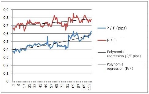
Fig. 12. Model profit factor charts on the sample of 118 bars
This chart represents the dependence of profit factors on the number of bars in the analysis. There is an obvious uptrend.
Let us check the results on the sample of 238 bars. The chart drawn is as follows:
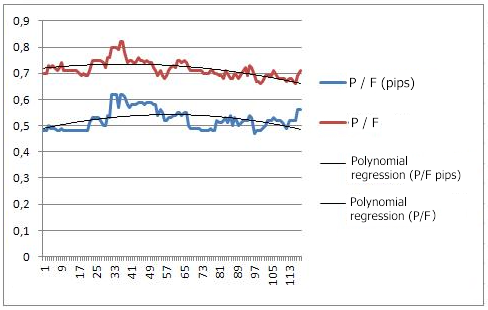
Fig. 13. Model profit factor charts on the sample of 236 bars
The fact that the profit factor charts differ suggests that the model is unstable.
Conclusion
The article has dealt with the use of one-step-ahead forecasts produced by EViews for the development of the Expert Advisor in MetaTrader 4.
The negative result we have obtained indicates that building a model in EViews is quite a complicated task which nevertheless appears to be more potentially productive than intuitive development of Expert Advisors.