Trader's Statistical Cookbook: Hypotheses

Denis Kirichenko | 10 February, 2015

Introduction

Any trader willing to create their own trading system is going to become an analyst sooner or later. They are permanently trying to find market trends and testing trading ideas. Testing an idea can be based on different approaches - from a usual search of best parameter values in the optimization mode of the Strategy Tester to scientific (sometimes pseudo scientific) market research.

In this article I suggest considering statistical hypothesis - an instrument of statistical analysis for research and inference verification. Let us test various hypotheses with the Statistica package and ported numerical analysis library ALGLIB MQL5 using examples.

1. The Concept of Hypothesis

There are several definitions of the "statistical hypothesis" concept. Some of them involve a supposition about statistical properties of the object or phenomenon under consideration.

Other definitions point out that the statistical properties must be connected with distribution of some random variable or parameters of this distribution.

In the literature on mathematical statistics, the notion of "hypothesis" is interpreted the second way. Then we can distinguish:

1. Parametric hypothesis (hypothesis about the values of distribution parameters or about comparative value of parameters of two distributions);
2. Nonparametric hypothesis (hypothesis about the type of a random value distribution).

In the next section we will discuss a method of hypothesis verification.

2. Testing Hypotheses. Theory

The hypothesis to be tested is called a null hypothesis (Н0). A competing hypothesis (Н1) is its alternative. It is on the flip side of the Н0's coin, i.e. it logically refuses the null hypothesis.

Imagine, that there is a population of data on Stop Losses of some trading system. We are going to state two hypotheses making a basis for testing.

Н0 – average Stop Loss value equal to 30 points;

Н1 – average Stop Loss value not equal to 30 points.

Variants of acceptance and rejection of hypotheses:

1. Н0 is true and it is accepted;
2. Н0 is wrong and it is rejected in favor of Н1;
3. Н0 is true but it is rejected in favor of Н1;
4. Н0 is wrong but it is accepted.

The last two variants are connected with errors.

Now the value of significance level is to be specified. It is the probability that the alternative hypothesis will be accepted whereas the true hypothesis is the null one (third variant). This probability is preferable to be minimized.

In our case such error will occur if we assume that Stop Loss at the average is not equal to 30 points even though that it actually is.

Usually the significance level (α) is equal to 0.05. That means that the test statistic value of the null hypothesis can populate the critical region in no more that 5 cases out of 100.

In our case the test statistic value will be evaluated on a classical chart (Fig.1).

Fig.1. Test statistic value distribution by normal probability law

For the null hypothesis to be accepted, the test statistic values are not supposed to get to the red zones. For the purpose of the example, let us assume that the test statistic values are distributed normally.

Every test has its own formula to calculate the test statistic value with.

Variant 4 implies that there is an error of the second type (β). In our case such an error will occur if we presume that Stop Loss at the average is equal to 30 points and it is not equal to that number of points.

3. Examples of Statistical Hypothesis Testing

The source data used for examples are stored in the Data.xls file.

3.1. Dependent Sample Testing

Imagine the following situation. Assume that there is a trading system generating a population of deals. Let us take a sample of profitable deals with volume of 100 units. The source data is in the "Profits" sheet.

Descriptive statistics of the Profits sample after deleting outlying cases are presented in Table 1:

Table 1. Statistics of the Profits sample

The sample histogram looks as follows (Fig.2).

Fig.2. The Profits sample histogram

The value of mean is 83.4 points and median is 83 points.

What will happen if the market entry point gets changed by a few points? For example, a limit order improving the entry price can be placed after a trade signal appears.

How will it affect the results? This question can be answered with statistical hypotheses.

In the Statistica package we formally check if the samples were not taken from one population:

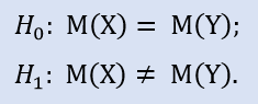
If we change the entry price by 15 points, we shall receive the NewProfits sample. Ideally the result picture should be as follows (Fig.3).

Fig.3. Chart for Profits and NewProfits samples

The probability that the alternative hypothesis will be accepted is high as the medians of samples differ.

This picture, however, will be difficult to obtain as there might be no better prices on the market. In my case, the second sample comprised 84 deals after the entry price was changed. The other 15 deals simply were not performed. This corrected sample will be named NewProfitsReal.

On the plot of the "box-and-whisker" type there is not much difference between two samples.

Fig.4. Plot for the Profits and NewProfitsReal samples

Let us conduct a nonparametric Wilcoxon signed-rank test for connected sample.

Results are in Table 2:

Table 2. Wilcoxon test results for the Profits and NewProfitsReal samples

Significance level is very high, which favors the null hypothesis.

This way we can tell that changing of the entry point did not influence the system yield. It is in relative terms. In absolute terms, the system turned out to be less profitable because of missed entry points.

Wilcoxon test can be conducted programmatically in MQL5. Although it compares the distribution median with the specified value of m, this difference is not significant.

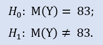
We are going to check:

The ALGLIB library contains the following procedure: CAlglib::WilcoxonSignedRankTest(). It gives a result for three test types: two-sided, left-sided and right-sided.

Script test_profits.mq5 provides an example of this calculation. The "Experts" journal has the following results for the NewProfitsReal sample:

OO      0       12:04:08.814    test_profits (EURUSD.e,H1)      p-value for the two-sided test: 0.7472
HD      0       12:04:08.814    test_profits (EURUSD.e,H1)      p-value for the left-sided test: 0.6285
CM      0       12:04:08.814    test_profits (EURUSD.e,H1)      p-value for the right-sided test: 0.3736

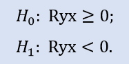
Left-sided test has the form of:

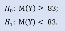
Here we check the alternative as the median of the NewProfitsReal sample can be greater or equal to 83. Error probability at rejecting H0 is 0.63. Therefore H0 is accepted.

Right-sided test looks like:

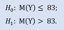
In this test we check the alternative that the median of the NewProfitsReal sample can be less or equal to 83. Error probability at rejecting H0 is equal to 0.37. Therefore H0 is accepted.

3.2. Testing Independent Samples

Let's assume that we have to check how quickly different brokers process trading orders and if there is a difference between brokers in relation to the execution time of trading orders.

So, there are two samples of source data for analysis. Every sample initially contained 50 observations. After deleting outlying cases, 48 observations were left in the first sample (broker А), and 49 observations in the second (broker B). Data can be found in the "ExecutionTime" sheet.

We are going to check:

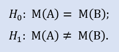
Let us represent sample indices on a picture (Fig.5). According to the plot, the values of the medians differ though not significantly.

Fig.5. Plot for the data samples of brokers A and B

Since we do not know what distribution every sample belongs to, we shall refer to nonparametric tests for comparison.

For example let us carry out Mann — Whitney U-test (Table 3). It is believed to be the most informative.

Table 3. Mann — Whitney U-test results for data samples of brokers A and B

Conclusion: test results differ and therefore the null hypotheses about equality of samples is rejected in favor to Н1.

Mann — Whitney U-test can be conducted programmatically in MQL5. In the ALGLIB library there is the CAlglib:: MannWhitneyUTest() procedure. It gives a result for three test types: two-sided, left-sided and right-sided.

Script test_time_execution.mq5 provides an example of calculation. The "Expert" journal has the following result that can be used for comparing samples:

MR      0       12:55:08.577    test_time_execution (EURUSD.e,H1)       p-value for the two sided test: 0.0001
QF      0       12:55:08.577    test_time_execution (EURUSD.e,H1)       p-value for the left-sided test: 1.0000
PF      0       12:55:08.577    test_time_execution (EURUSD.e,H1)       p-value for the right-sided test: 0.0001

Left-sided test has the form of:

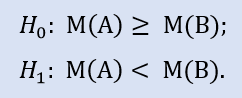
The null hypothesis is that the median of broker A data sample can be greater or equal to the median of broker B data sample. The alternative is its rejection. Error probability at rejecting H0 is 1.0. Therefore H0 is accepted.

Right-sided test looks like:

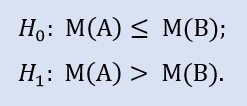
The null hypothesis is that the median of broker A data sample can be less or equal to the median of broker B data sample. The alternative is its rejection.

Error probability at rejecting H0 is 0.0. Therefore H0 is rejected in favor of Н1.

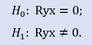
3.3. Correlation Test

Imagine a portfolio of strategies. The goal is to reduce the number of strategies in the portfolio.

The choice criterion will be as follows: if two strategies are the same at comparing Stop Loss series, then one of the strategies will be removed from the portfolio. Let us take two samples with Stop Loss data of two different systems. Assumption: systems react at market entry the same way and react exiting the market differently.

We are going to use Spearman's Rank-Order Correlation test. There are three samples in "Correlation" sheet of the data file.

Check if the correlation coefficient is equal to zero:

Comparison of the pair of the Stops1-Stops2 samples will give the following result (Table 4).

Table 4. Spearman's Rank-Order Correlation test for the Stops1 and Stops2 samples

In this case the null hypothesis about absence of connection between elements of samples cannot be rejected in favor to the alternative. Therefore it is accepted.

The plot on Fig.6 shows that data does not form any noticeable configuration. The data is scattered on the plot plane.

Fig.6. Scatter plot for the Stops1 and Stops2 samples

Results of a relationship check between the Stops1-Stops3 samples are shown in Table 5:

Table 5. Results of the Spearman's Rank-Order Correlation test for the Stops1 and Stops3 samples

In this case the null hypothesis can be rejected as probability of an error is very low.

Hence, the alternative about an existing relationship is accepted. The relationship looks like (Fig.7).

Fig.7. Scatter plot for the Stops1 and Stops3 samples

Confirm the result with the code in MQL5. The test_correlation.mq5 contains a calculation example.

The ALGLIB library contains procedure CAlglib::SpearmanRankCorrelationSignificance(), which implements the test for significance of Spearman's Rank-Order Correlation coefficient.

The journal contains the following records:

OO      0       12:57:43.545    test_correlation (EURUSD.e,H1)  ---===Samples Stops1 and Stops2===---
GO      0       12:57:43.545    test_correlation (EURUSD.e,H1)  p-value for the two-sided test: 0.9840
KK      0       12:57:43.545    test_correlation (EURUSD.e,H1)  p-value for the left-sided test: 0.4920
JJ      0       12:57:43.545    test_correlation (EURUSD.e,H1)  p-value for the right-sided test: 0.5080
DM      0       12:57:43.545    test_correlation (EURUSD.e,H1)  
HJ      0       12:57:43.545    test_correlation (EURUSD.e,H1)  ---===Samples Stops1 and Stops3===---
NS      0       12:57:43.545    test_correlation (EURUSD.e,H1)  p-value for the two-sided test: 0.0002
RO      0       12:57:43.545    test_correlation (EURUSD.e,H1)  p-value for the left-sided test: 0.9999
FG      0       12:57:43.545    test_correlation (EURUSD.e,H1)  p-value for the right-sided test: 0.0001

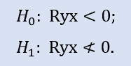
Left-sided test has the form of:

In this test the null hypothesis that there is a non-negative correlation between variables (i.e. the correlation is either zero, or negative) is verified.

The left-sided test shows that for the pair of samples Stops1-Stops2, the zero hypothesis is accepted. The left-sided test shows that for the pair of samples Stops1-Stops3 the null hypothesis is accepted too. A logical question to ask will be "Why is there no connection between the Stops1-Stops2 samples and there is one between Stops1-Stops3?" The reason is that the statement in check is "greater or equal to zero". In the first case, "equal to zero" is important for H0, and in the second case it is "greater than zero".

Right-sided test looks like:

Here, the null hypothesis of what is a negative correlation is checked.

For the pair of samples Stops1-Stops2, the right-sided test shows that the null hypothesis is accepted. For the pair of samples Stops1-Stops3 the right-sided test shows that the null hypothesis is rejected.

One last comment. The test revealed that there is a positive probabilistic connection between the samples of Stops1-Stops3. The strength of this connection is average. Therefore it is up to trader to decide whether to reject strategy 1 or 3.

Conclusion

In this article I tried to show on examples that quantitative variables can be assessed using mathematical statistics. I hope that novice developers will find this article useful for their future trading systems. I also hope that the series of articles about using methods of mathematical statistics will be continued.

Files of the ALGLIB library need to be downloaded separately.