Data Science and Machine Learning (Part 13): Improve your financial market analysis with Principal Component Analysis (PCA)

Omega J Msigwa | 20 March, 2023

"PCA is a fundamental technique in data analysis and machine learning, and is widely used in applications ranging from image and signal processing to finance and social sciences."

David J. Sheskin

Introduction

Principal Component Analysis (PCA) is a dimensionality-reduction method that is often used to reduce the dimensionality of large data sets, by transforming a large set of variables into a smaller one that still contains most of the information in the large set.

Reducing the number of variables in the dataset usually comes at the expense of accuracy, but the trick in dimensionality reduction is to trade little accuracy for simplicity. You and I both know that a few variables in the dataset are easier to explore, visualize and make analyzing data much easier and faster for machine learning algorithms. I personally don't think trading simplicity for accuracy is a bad thing at all because we are in the trading space. Accuracy doesn't necessarily mean profits.

The main idea of PCA is very simple at the core: Reduce the number of variables in a data set, while preserving as much information as possible. Let's look at the steps involved in the Principal Component Analysis algorithm.

Steps Involved in the Principal Component Analysis Algorithm

Standardizing the data
Finding the Covariance of the matrix
Finding eigenvectors & eigen values
Finding the PCA scores & Standardizing them
Obtaining the components

Without further ado, let's start by Standardizing the Data.

01: Standardizing the Data

The purpose of standardizing the data is to bring all the variables to the same scale so that they are compared and analyzed on an equal footing. When analyzing data, it is often the case that the variables have different units or scales of measurement which can lead to biased results or incorrect conclusions. For example, the Moving Average indicator has the price range same as the market value, meanwhile the RSI indicator has values typically between 0 and 100. These two variables will be incomparable when used together in any model. They can not be used together in a meaningful way.

Standardizing the data involves transforming each variable so that it has a mean of zero and as tandard deviation of one. This ensures that each variable has the same scale and distribution, making them directly comparable. Standardizing the data can also help to improve the accuracy and stability of machine learning models, especially when the variables have different magnitudes or variances.

To demonstrate a point, I am going to be using the blood pressure data. I usually use different sorts of irrelevant data just to build things up because this kind of data is human-relatable so it makes it easier to understand and debug stuff.

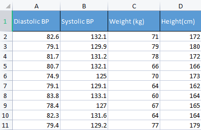
   matrix Matrix = matrix_utiils.ReadCsv("bp data.csv");

   pre_processing = new CPreprocessing(Matrix, NORM_STANDARDIZATION);

Before and after:

CS      0       10:17:31.956    PCA Test (NAS100,H1)    Non-Standardized data
CS      0       10:17:31.956    PCA Test (NAS100,H1)    [[82.59999999999999,132.1,71,172]
CS      0       10:17:31.956    PCA Test (NAS100,H1)     [79.09999999999999,129.9,79,180]
CS      0       10:17:31.956    PCA Test (NAS100,H1)     [81.7,131.2,78,172]
CS      0       10:17:31.956    PCA Test (NAS100,H1)     [80.7,132.1,66,166]
CS      0       10:17:31.956    PCA Test (NAS100,H1)     [74.90000000000001,125,70,173]
CS      0       10:17:31.956    PCA Test (NAS100,H1)     [79.09999999999999,129.1,64,162]
CS      0       10:17:31.956    PCA Test (NAS100,H1)     [83.8,133.1,60,164]
CS      0       10:17:31.956    PCA Test (NAS100,H1)     [78.40000000000001,127,67,165]
CS      0       10:17:31.956    PCA Test (NAS100,H1)     [82.3,131.6,64,164]
CS      0       10:17:31.956    PCA Test (NAS100,H1)     [79.40000000000001,129.2,77,179]]
CS      0       10:17:31.956    PCA Test (NAS100,H1)    Standardized data
CS      0       10:17:31.956    PCA Test (NAS100,H1)    [[0.979632638610581,0.8604038253411385,0.2240645398825688,0.3760399462363875]
CS      0       10:17:31.957    PCA Test (NAS100,H1)     [-0.4489982926965129,-0.0540350228475094,1.504433339211528,1.684004976623816]
CS      0       10:17:31.957    PCA Test (NAS100,H1)     [0.6122703991316175,0.4863152056275964,1.344387239295408,0.3760399462363875]
CS      0       10:17:31.957    PCA Test (NAS100,H1)     [0.2040901330438764,0.8604038253411385,-0.5761659596980309,-0.6049338265541837]
CS      0       10:17:31.957    PCA Test (NAS100,H1)     [-2.163355410265021,-2.090739730176784,0.06401843996644889,0.539535575034816]
CS      0       10:17:31.957    PCA Test (NAS100,H1)     [-0.4489982926965129,-0.3865582403706605,-0.8962581595302708,-1.258916341747898]
CS      0       10:17:31.957    PCA Test (NAS100,H1)     [1.469448957915872,1.276057847245071,-1.536442559194751,-0.9319250841510407]
CS      0       10:17:31.957    PCA Test (NAS100,H1)     [-0.7347244789579271,-1.259431686368917,-0.416119859781911,-0.7684294553526122]
CS      0       10:17:31.957    PCA Test (NAS100,H1)     [0.8571785587842599,0.6525768143891719,-0.8962581595302708,-0.9319250841510407]
CS      0       10:17:31.957    PCA Test (NAS100,H1)     [-0.326544212870186,-0.3449928381802696,1.184341139379288,1.520509347825387]]

In the context of Principal Component Analysis(PCA), standardizing the data is an essential step because PCA is based on the covariance matrix, which is sensitive to differences in scale and variance between the variables. Standardizing the data before running the PCA ensures that the resulting principal components are not dominated by the variables with larger magnitude or variances, which could distort the analysis and lead to erroneous conclusions.

02: Finding the Covariance of the Matrix

Covariance Matrix is a matrix that contain the measurement of how much random variables affect change together. It is used for computing the covariance in between every column of the data matrix. The covariance between two jointly distributed real-valued random variables X and Y with finite second moments is defined as:

But, you don't have to worry about understanding this formula since the Standard library has this function.

   matrix Cova = Matrix.Cov(false);

   Print("Covariances\n", Cova);

Outputs:

CS      0       10:17:31.957    PCA Test (NAS100,H1)    Covariances
CS      0       10:17:31.957    PCA Test (NAS100,H1)    [[1.111111111111111,1.05661579634328,-0.2881675653452953,-0.3314539233600543]
CS      0       10:17:31.957    PCA Test (NAS100,H1)     [1.05661579634328,1.111111111111111,-0.2164241126576326,-0.2333966556085017]
CS      0       10:17:31.957    PCA Test (NAS100,H1)     [-0.2881675653452953,-0.2164241126576326,1.111111111111111,1.002480628180182]
CS      0       10:17:31.957    PCA Test (NAS100,H1)     [-0.3314539233600543,-0.2333966556085017,1.002480628180182,1.111111111111111]]

Beware that the covariance is a square matrix with values of 1 on the diagonal. When calling this covariance matrix method you have to set the rowval input to false.

matrix matrix::Cov( 
  const bool    rowvar=true  // rows or cols vectors of observations 
);

because we want our square matrix to be an identity matrix based on the columns we give this function, since we have 4 columns. The output will be 4x4 matrix otherwise It would have been a 8x8 matrix.

03: Finding Eigenvectors and Eigen values

Eigen vector, also known as eigenvectors, are special vectors that are associated with a square matrix. An eigenvector of a matrix is a non-zero vector that, when multiplied by the matrix, results in a scalar multiple of itself, called eigenvalue.

More formally, if A is a square matrix, then a non zero vector v is an eigenvector of A if there exists a scalar λ, called the eigenvalue such that; Av = λv. For more details read.

No need to worry about understanding the formulas for this either, it is also in the standard library.

   if (!Cova.Eig(component_matrix, eigen_vectors))
      Print("Failed to get the Component matrix matrix & Eigen vectors");

If you take a closer look at this Eig method.

bool matrix::Eig( 
  matrix&  eigen_vectors,     // matrix of eigenvectors  
  vector&  eigen_values       // vector of eigenvalues  
   );

You may notice the first input matrix eigen_vectors returns eigen vectors, just as labelled. But this eigen vector can also be referred to as the component matrix. So I am storing this eigenvectors in the component matrix as I find it confusing to call it eigenvector when in reality it is a matrix, according to the MQL5 language standards.

Print("\nComponent matrix\n",component_matrix,"\nEigen Vectors\n",eigen_vectors);

Outputs:

CS      0       10:17:31.957    PCA Test (NAS100,H1)    Component matrix
CS      0       10:17:31.957    PCA Test (NAS100,H1)    [[-0.5276049902734494,0.459884739531444,0.6993704635263588,-0.1449826035480651]
CS      0       10:17:31.957    PCA Test (NAS100,H1)     [-0.4959779194731578,0.5155907011803843,-0.679399121133044,0.1630612352922813]
CS      0       10:17:31.957    PCA Test (NAS100,H1)     [0.4815459137666799,0.520677926282417,-0.1230090303369406,-0.6941734714553853]
CS      0       10:17:31.957    PCA Test (NAS100,H1)     [0.4937128827246101,0.5015643052337933,0.184842006606018,0.6859404272536788]]
CS      0       10:17:31.957    PCA Test (NAS100,H1)    Eigen Vectors
CS      0       10:17:31.957    PCA Test (NAS100,H1)    [2.677561590453738,1.607960239905343,0.04775016337426833,0.1111724507110918]

05: Finding the PCA scores.

Finding the Principal Component Analysis scores is very easy and takes a single line of code.

 pca_scores = Matrix.MatMul(component_matrix);

The PCA scores can be found by multiplying the Normalized matrix by the component matrix.

Outputs:

CS      0       10:17:31.957    PCA Test (NAS100,H1)    PCA SCORES
CS      0       10:17:31.957    PCA Test (NAS100,H1)    [[-0.6500472384886967,1.199407986803537,0.1425145462368588,0.1006701620494091]
CS      0       10:17:31.957    PCA Test (NAS100,H1)     [1.819562596624738,1.393614599196321,-0.1510888243020112,0.1670753033981925]
CS      0       10:17:31.957    PCA Test (NAS100,H1)     [0.2688014256048517,1.420914385142756,0.001937917070391801,-0.6847663538666366]
CS      0       10:17:31.957    PCA Test (NAS100,H1)     [-1.110534258768705,-0.06593596223641518,-0.4827665581567511,0.09571954869438426]
CS      0       10:17:31.957    PCA Test (NAS100,H1)     [2.475561333978323,-1.768915328424386,-0.0006861487484489809,0.2983796568520111]
CS      0       10:17:31.957    PCA Test (NAS100,H1)     [-0.6245145789301378,-1.503882637300733,-0.1738415909335406,-0.2393186981373224]
CS      0       10:17:31.957    PCA Test (NAS100,H1)     [-2.608156175249579,0.0662886285379769,0.1774740257067155,0.4223436077935874]
CS      0       10:17:31.957    PCA Test (NAS100,H1)     [0.4325302694103054,-1.589321053467977,0.2509606394263523,-0.337079680008286]
CS      0       10:17:31.957    PCA Test (NAS100,H1)     [-1.667608250048573,-0.2034163217366656,0.09411419638842802,-0.03495245015036286]
CS      0       10:17:31.957    PCA Test (NAS100,H1)     [1.664404875867474,1.051245703485609,0.1413817973120564,0.2119289033750197]]

Once we have the PCA scores we need to standardize them.

   pre_processing = new CPreprocessing(pca_scores_standardized, NORM_STANDARDIZATION);

Outputs:

CS      0       10:17:31.957    PCA Test (NAS100,H1)    PCA SCORES | STANDARDIZED
CS      0       10:17:31.957    PCA Test (NAS100,H1)    [[-0.4187491401035159,0.9970295470975233,0.68746486754918,0.3182591681100855]
CS      0       10:17:31.957    PCA Test (NAS100,H1)     [1.172130620033975,1.15846730049564,-0.7288256625700642,0.528192723531639]
CS      0       10:17:31.957    PCA Test (NAS100,H1)     [0.1731572094549987,1.181160740523977,0.009348167869829477,-2.164823873278453]
CS      0       10:17:31.957    PCA Test (NAS100,H1)     [-0.715386880184365,-0.05481045923432144,-2.328780161211247,0.3026082735855334]
CS      0       10:17:31.957    PCA Test (NAS100,H1)     [1.594713612332284,-1.470442808583469,-0.003309859736641006,0.9432989819176616]
CS      0       10:17:31.957    PCA Test (NAS100,H1)     [-0.4023014443028848,-1.250129598312728,-0.8385809690405054,-0.7565833632510734]
CS      0       10:17:31.957    PCA Test (NAS100,H1)     [-1.68012890598631,0.05510361946569121,0.8561031894464458,1.335199254045385]
CS      0       10:17:31.957    PCA Test (NAS100,H1)     [0.2786284867625921,-1.321151824538665,1.210589566461227,-1.06564543418136]
CS      0       10:17:31.957    PCA Test (NAS100,H1)     [-1.074244269325531,-0.1690934905926844,0.4539901733759543,-0.1104988556867913]
CS      0       10:17:31.957    PCA Test (NAS100,H1)     [1.072180711318756,0.8738669736790375,0.6820006878558206,0.6699931252073736]]

06: Obtaining the PCA Components

Last but not least, we need to obtain the Principal components which is the purpose of all those steps we were doing.

To be able to obtain the components we need to find the coefficients of non-standardized PCA scores, remember!! we now have two PCA scores, the standardized-one and non-standardized one.

The Coefficients of each PCA score is just the variance of each column in the PCA scores column.

   pca_scores_coefficients.Resize(cols);
   vector v_row;
   
   for (ulong i=0; i<cols; i++)
     {
       v_row = pca_scores.Col(i);
       
       pca_scores_coefficients[i] = v_row.Var(); //variance of the pca scores
     }

Outputs:

2023.02.25 10:17:31.957 PCA Test (NAS100,H1)    SCORES COEFF [2.409805431408367,1.447164215914809,0.04297514703684173,0.1000552056399828]

To extract the Principal components there are criteria we need to consider among many:

Eigenvalue criterion: This criterion involves selecting the principal components with the largest eigenvalues. The idea is that the largest eigenvalues correspond to the principal components that capture the most variance in the data.
The Proportion of Variance criterion: This criterion involves selecting the principal components that explain a certain proportion of the total variance in the data. In this library, I'm going to set it to greater than 90%.
Scree plot criterion: This criterion involves examining the scree plot, which shows the eigen-values of each principal component in descending order. The point at which the curve starts to level off is used as a threshold for selecting the principal components to retain.
Kaiser criterion: This criterion involves retaining only the principal components with eigen-values greater than the Mean of the coefficients. In other words the principal component with coefficients greater than one.
Cross-validation criterion: This criterion involves evaluating the performance of the PCA model on a validation set, and selecting the principal components that yield the best predictive accuracy.

In this library I have coded for three criteria that I think are better and computationally efficient. They are Proportion of variance, Kaiser, and Scree plot. You can choose each one of them using from the below enum;

enum criterion
  {
    CRITERION_VARIANCE,
    CRITERION_KAISER,
    CRITERION_SCREE_PLOT
  };

Below is the complete function for extracting the principal components:

matrix Cpca::ExtractComponents(criterion CRITERION_)
 {

  vector vars = pca_scores_coefficients;   
  vector vars_percents = (vars/(double)vars.Sum())*100.0;
  
//--- for Kaiser
  double vars_mean = pca_scores_coefficients.Mean();

//--- for scree 
   double x[], y[];
   
//---
  matrix PCAS = {};
  
  double sum=0;
  ulong  max;
  vector v_cols = {};
   
   switch(CRITERION_)
     {
      case  CRITERION_VARIANCE:       
       #ifdef DEBUG_MODE
        Print("vars percentages ",vars_percents);       
       #endif  
     
         for (int i=0, count=0; i<(int)cols; i++)
           { 
             count++;
             
              max = vars_percents.ArgMax();
              sum += vars_percents[max];
              
              vars_percents[max] = 0; 
              
              v_cols.Resize(count);
              v_cols[count-1] = (int)max;
                   
              if (sum >= 90.0)
		 break;
           }
         
         PCAS.Resize(rows, v_cols.Size());
         
         for (ulong i=0; i<v_cols.Size(); i++)
            PCAS.Col(pca_scores.Col((ulong)v_cols[i]), i);
         
        break;
      case  CRITERION_KAISER:
      
      #ifdef DEBUG_MODE
         Print("var ",vars," scores mean ",vars_mean);
      #endif 
      
       vars = pca_scores_coefficients;
        for (ulong i=0, count=0; i<cols; i++)
           if (vars[i] > vars_mean)
             {
               count++;
       
               PCAS.Resize(rows, count);
               
               PCAS.Col(pca_scores.Col(i), count-1);
             }           
           
        break;
      case  CRITERION_SCREE_PLOT:        
         v_cols.Resize(cols);     
         for (ulong i=0; i<v_cols.Size(); i++)
             v_cols[i] = (int)i+1;
             
         
          vars = pca_scores_coefficients;          
          SortAscending(vars); //Make sure they are in ascending first order
          ReverseOrder(vars);  //Set them to descending order
          
          VectorToArray(v_cols, x);
          VectorToArray(vars, y);
          
          plt.ScatterCurvePlots("Scree plot",x,y,"variance","PCA","Variance");

//---
       vars = pca_scores_coefficients;
        for (ulong i=0, count=0; i<cols; i++)
           if (vars[i] > vars_mean)
             {
               count++;       
               PCAS.Resize(rows, count);       
               PCAS.Col(pca_scores.Col(i), count-1);
             }    
             
        break;
     } 
   return (PCAS);
 }

Since the Kaiser criterion is set to select the Principal components with coefficients that explain up to more than 90% of all variances. I had to convert the variances into percentages:

  vector vars = pca_scores_coefficients;   
  vector vars_percents = (vars/(double)vars.Sum())*100.0;

Below are the outputs using each method.

CRITERION KAISER:

CS      0       12:03:49.579    PCA Test (NAS100,H1)    PCA'S
CS      0       12:03:49.579    PCA Test (NAS100,H1)    [[-0.6500472384886967,1.199407986803537]
CS      0       12:03:49.579    PCA Test (NAS100,H1)     [1.819562596624738,1.393614599196321]
CS      0       12:03:49.579    PCA Test (NAS100,H1)     [0.2688014256048517,1.420914385142756]
CS      0       12:03:49.579    PCA Test (NAS100,H1)     [-1.110534258768705,-0.06593596223641518]
CS      0       12:03:49.579    PCA Test (NAS100,H1)     [2.475561333978323,-1.768915328424386]
CS      0       12:03:49.579    PCA Test (NAS100,H1)     [-0.6245145789301378,-1.503882637300733]
CS      0       12:03:49.579    PCA Test (NAS100,H1)     [-2.608156175249579,0.0662886285379769]
CS      0       12:03:49.579    PCA Test (NAS100,H1)     [0.4325302694103054,-1.589321053467977]
CS      0       12:03:49.579    PCA Test (NAS100,H1)     [-1.667608250048573,-0.2034163217366656]
CS      0       12:03:49.579    PCA Test (NAS100,H1)     [1.664404875867474,1.051245703485609]]

CRITERION VARIANCE:

CS      0       12:03:49.579    PCA Test (NAS100,H1)    PCA'S
CS      0       12:03:49.579    PCA Test (NAS100,H1)    [[-0.6500472384886967,1.199407986803537]
CS      0       12:03:49.579    PCA Test (NAS100,H1)     [1.819562596624738,1.393614599196321]
CS      0       12:03:49.579    PCA Test (NAS100,H1)     [0.2688014256048517,1.420914385142756]
CS      0       12:03:49.579    PCA Test (NAS100,H1)     [-1.110534258768705,-0.06593596223641518]
CS      0       12:03:49.579    PCA Test (NAS100,H1)     [2.475561333978323,-1.768915328424386]
CS      0       12:03:49.579    PCA Test (NAS100,H1)     [-0.6245145789301378,-1.503882637300733]
CS      0       12:03:49.579    PCA Test (NAS100,H1)     [-2.608156175249579,0.0662886285379769]
CS      0       12:03:49.579    PCA Test (NAS100,H1)     [0.4325302694103054,-1.589321053467977]
CS      0       12:03:49.579    PCA Test (NAS100,H1)     [-1.667608250048573,-0.2034163217366656]
CS      0       12:03:49.579    PCA Test (NAS100,H1)     [1.664404875867474,1.051245703485609]]

CRITERION SCREE PLOT:

Great so now we have two Principal components. In simple language, the dataset is reduced from 4 variables to only 2 variables. You can then use these variables in whatever project you were working on.

Principal Component Analysis in MetaTrader

Now, it's time to use Principal component Analysis on what you want to see, the trading environment.

To do that I picked up 10 oscillators. Since they are all oscillators, I decided to give them a shot when trying to prove a point, that if you have 10 indicators of the same type you can do PCA to reduce them so that you end up with a few variables that are easy to work with.

I added 10 indicators to a single chart which are: ATR, Bears Power, MACD, Chaikin Oscillator, Commodity Channel Index, De marker, force index, Momentum, RSI, Williams percent range.

   handles[0] = iATR(Symbol(),PERIOD_CURRENT, period);
   handles[1] = iBearsPower(Symbol(), PERIOD_CURRENT, period);
   handles[2] = iMACD(Symbol(),PERIOD_CURRENT,12, 26,9,PRICE_CLOSE);
   handles[3] = iChaikin(Symbol(), PERIOD_CURRENT,12,26,MODE_SMMA,VOLUME_TICK);
   handles[4] = iCCI(Symbol(),PERIOD_CURRENT,period, PRICE_CLOSE);
   handles[5] = iDeMarker(Symbol(),PERIOD_CURRENT,period);
   handles[6] = iForce(Symbol(),PERIOD_CURRENT,period,MODE_EMA,VOLUME_TICK);
   handles[7] = iMomentum(Symbol(),PERIOD_CURRENT,period, PRICE_CLOSE);
   handles[8] = iRSI(Symbol(),PERIOD_CURRENT,period,PRICE_CLOSE);
   handles[9] = iWPR(Symbol(),PERIOD_CURRENT,period);
   
   
   for (int i=0; i<10; i++)
    {
      matrix_utiils.CopyBufferVector(handles[i],0,0,bars,buff_v);
      ind_Matrix.Col(buff_v, i); //store each indicator in ind_matrix columns
    }

I decided to visualize all these indicators the same chart. Below is how they look:

How on earth do they all look nearly the same, Let's see their correlation matrix:

    Print("Oscillators Correlation Matrix\n",ind_Matrix.CorrCoef(false));

Outputs:

CS      0       18:03:44.405    PCA Test (NAS100,H1)    Oscillators Correlation Matrix
CS      0       18:03:44.405    PCA Test (NAS100,H1)    [[1,0.01772984879133655,-0.01650305145071043,0.03046861668248528,0.2933315924162302,0.09724971519249033,-0.054459564042778,-0.0441397473782667,0.2171969726706487,0.3071254662907512]
CS      0       18:03:44.405    PCA Test (NAS100,H1)     [0.01772984879133655,1,0.6291675928958272,0.2432064602541826,0.7433991440764224,0.7857575973967624,0.8482060554701495,0.8438879842180333,0.8287766948950483,0.7510097635884428]
CS      0       18:03:44.405    PCA Test (NAS100,H1)     [-0.01650305145071043,0.6291675928958272,1,0.80889919514547,0.3583185473647767,0.79950773673123,0.4295059398014639,0.7482107564439531,0.8205910850439753,0.5941794310595322]
CS      0       18:03:44.405    PCA Test (NAS100,H1)     [0.03046861668248528,0.2432064602541826,0.80889919514547,1,0.03576792595345671,0.436675349452699,0.08175026884450357,0.3082792264724234,0.5314362133025707,0.2271361556104472]
CS      0       18:03:44.405    PCA Test (NAS100,H1)     [0.2933315924162302,0.7433991440764224,0.3583185473647767,0.03576792595345671,1,0.6368513319457978,0.701918992559641,0.6677393692960837,0.7952832674277922,0.8844891719743937]
CS      0       18:03:44.405    PCA Test (NAS100,H1)     [0.09724971519249033,0.7857575973967624,0.79950773673123,0.436675349452699,0.6368513319457978,1,0.6425071357003039,0.9239712092224102,0.8809179254503203,0.7999862160768584]
CS      0       18:03:44.405    PCA Test (NAS100,H1)     [-0.054459564042778,0.8482060554701495,0.4295059398014639,0.08175026884450357,0.701918992559641,0.6425071357003039,1,0.7573281438252102,0.7142333470379938,0.6534102287503526]
CS      0       18:03:44.405    PCA Test (NAS100,H1)     [-0.0441397473782667,0.8438879842180333,0.7482107564439531,0.3082792264724234,0.6677393692960837,0.9239712092224102,0.7573281438252102,1,0.8565660350098397,0.8221821793990941]
CS      0       18:03:44.405    PCA Test (NAS100,H1)     [0.2171969726706487,0.8287766948950483,0.8205910850439753,0.5314362133025707,0.7952832674277922,0.8809179254503203,0.7142333470379938,0.8565660350098397,1,0.8866871375902136]
CS      0       18:03:44.405    PCA Test (NAS100,H1)     [0.3071254662907512,0.7510097635884428,0.5941794310595322,0.2271361556104472,0.8844891719743937,0.7999862160768584,0.6534102287503526,0.8221821793990941,0.8866871375902136,1]]

Looking at the correlation matrix you may notice that it is only a few indicators that correlate to some others but they are the minority so they don't look the same after all. Let us apply the PCA to this matrix and see what this algorithm got for us.

    pca = new Cpca(ind_Matrix);
    matrix pca_matrix = pca.ExtractComponents(ENUM_CRITERION);

I chose the scree plot criterion below is the plot:

Looking at the scree plot, it's undeniable that 3 PCA(s) only have been selected, below is how they look;

CS      0       15:03:30.992    PCA Test (NAS100,H1)    PCA'S
CS      0       15:03:30.992    PCA Test (NAS100,H1)    [[-2.297373513063062,0.8489493134565058,0.02832445955171548]
CS      0       15:03:30.992    PCA Test (NAS100,H1)     [-2.370488225540198,0.9122356709081817,-0.1170316144060158]
CS      0       15:03:30.992    PCA Test (NAS100,H1)     [-2.728297784013197,1.066014896296926,-0.2859442064697605]
CS      0       15:03:30.992    PCA Test (NAS100,H1)     [-1.818906988827231,1.177846546204641,-0.748128826146959]
...
...
CS      0       15:03:30.992    PCA Test (NAS100,H1)     [-3.26602969252589,0.4816995789189212,-0.7408982990360158]
CS      0       15:03:30.992    PCA Test (NAS100,H1)     [-3.810781495417407,0.4426824869307094,-0.5737277071364888…]

From 10 variables to 3 variables only huh!!.

That's why it's very important to be a data analyst and a trader because I have seen traders having a lot of indicators on the chart and sometimes on Expert Advisors, I think using this way to reduce the variables is worth it in terms of decreasing the computation cost on our programs, by the way, this is not a piece of trading advice if what you've been doing works for you and you satisfied then there is nothing to worry about.

Let's visualize these Principal components to see how they look on the same axis.

       plt.ScatterCurvePlotsMatrix("pca's ",pca_matrix,"var","PCA");

Outputs:

Advantages of Principal Component Analysis

Dimensionality reduction: PCA can effectively reduce the number of variables in the dataset while retaining the most important information. This can simplify data analysis and visualization, reduce computational complexity, and improve model performance.
Data compression: PCA can be used to effectively compress large datasets into a smaller number of principal components, which can save storage space and reduce data transfer times.
Noise reduction: PCA can remove noise or random variation in the data by focusing on the most significant patterns or trends. As you just saw 10 oscillators had a lot of noise.
Interpretable results: PCA produces principal components that can be easily interpreted and visualized, which can aid in understanding the structure of the data.
Data normalization: PCA standardizes the data by scaling it to unit variance, which can reduce the impact of differences in variable scales and improve the accuracy of statistical models.

Disadvantages of the Principal Component Analysis.

Loss of information: PCA can lead to a loss of information if too many principal components are discarded or if the retained components do not capture all the relevant variations in the data.
Interpretation of results can be annoying: The interpretation of principal components can be difficult because you have no clue what are they just variables, especially when the original variables are highly correlated or when the number of principal components is large.
Sensitive to outliers: Just like a lot of ML techniques, outliers can distort this algorithm and lead to biased results.
Computationally intensive: In large dataset the PCA algorithm may create the same problem it's trying to solve.
Model assumptions: This algorithm assumes that the data is linearly related and the principal components are uncorrelated, which is not always true in practice. Violation of these assumptions can lead to poor results

Ending Remarks

in conclusion, Principal component Analysis (PCA) is a powerful technique that can be used to reduce the dimensionality of data while preserving the most important information. By identifying the principal components of a dataset, we can gain insight into the underlying structures of the market. PCA has a wide range of applications outside the trading field such as engineering and biology, Although it is a mathematically intensive technique, its benefits make it worth a shot. With the right approach and data, PCA can help us unlock new insights and make informed trading decisions based on the data we may have.

Track the development and changes of this algorithm on my GitHub Repo: https://github.com/MegaJoctan/MALE5

File	Descriptions
matrix_utils.mqh	Contains additional matrix manipulation functions
pca.mqh	The main Principal Component Analysis library
plots.mqh	Contains the class to aid in drawing vectors
preprocessing.mqh	library for preparing and scaling the data for ML algorithms
PCA Test.mqh	The EA for testing the Algorithm and everything discussed in this article

Reference Articles:

Matrix Utils, Extending the Matrices and Vector Standard Library Functionality