Data Science and Machine Learning (Part 12): Can Self-Training Neural Networks Help You Outsmart the Stock Market?
Omega J Msigwa | 13 March, 2023
“I’m not suggesting that neural networks are easy. You need to be an expert to make these things work. But that expertise serves you across a broader spectrum of applications. In a sense, all of the effort that previously went into feature design now goes into architecture design and loss function design and optimization scheme design. The manual labor has been raised to a higher level of abstraction.”
Stefano Soatto
Introduction
If you have been an algorithmic-trader for a while, chances are high you've heard about Neural Networks. It always seems like they are a way forward to make holy grails trading robots, about this I'm not that sure because it takes more than just adding neural networks to a trading bot to end up with a profitable system. Not to mention you need to understand what you are getting yourself into when using neural networks because even smaller details could mean a success or failure, i.e. profits or losses.

Honestly, I think neural nets are not going to work for anyone especially if you are not willing to get your hands dirty, because very often you need to spend time analyzing the errors produced by the model, pre-processing and scaling the input data, and much more stuff that I am going to be talking about in this article.
Let's kick off this article with a definition of an Artificial Neural network.
What is an Artificial Neural Network?
Simply put, an Artificial Neural Network, usually referred to as the neural network, is a computing system inspired by the biological neural networks that constitute animals' brains. To understand the basic components of a neural network, refer to this previous article of this series.
In the previous articles concerning neural networks, I explain the basic stuff concerning a feed-forward neural network. In this article, we will be exploring both the forward pass of a neural network and a backward pass, neural network training and testing. We will also create a trading robot based on the everything discussed lastly and will see how our trading robot performs.
In a multi-layer perceptron neural network, all neurons/nodes of a current layer are interconnected to the nodes of the second layer and so on, for all the layers from input to the output. This is what makes neural networks capable of figuring out complex relationships in the datasets. The more layers you have, the more your model is be capable of understanding complex relationships in the datasets. This comes at a high computational price to pay and may not necessarily guarantee model accuracy especially if the model is overcomplicated while the problem is a simple one.
In most cases, a single hidden layer is sufficient for the majority of problems people are trying to solve using these fancy neural networks. That's why we are going to use a single-layered neural network.
The Forward Pass
The operations involved in the forward pass are simple and can be achieved with a few lines of code. However, to make your neural networks flexible, you need to have a solid understanding of matrix and vector operations because they are the building block of neural networks and many machine learning algorithms we discuss in this series.
One important thing one needs to know is the type of problem they are trying to solve using neural network because different problems require different types of neural networks with different configurations and different outputs.
For those who don't know the types of problems below are
- Regression Problems
- Classification Problems
Regression problems are the kind of problems where we are trying to predict continuous variables, for example in trading we often try to predict the next price point the market will head on. I recommend reading Linear Regression for those who haven't yet.
These kinds of problems are tackled by regressor neural networks.
02: Classification Problems
Classification problems are the sort of problems in which we are trying to predict discrete/ non-continuous variables. In trading we could be predicting the signals, say 0 signal meaning the market heads down while 1 meaning the market heads up.
These kinds of problems are tackled by classification neural networks or Pattern recognition neural networks, in MATLAB they are referred to as patternnets
I will be solving a regression problem in this article by trying to predict the next price the market will move to.
matrix CRegNeuralNets::ForwardPass(vector &input_v)
 {
   matrix INPUT = this.matrix_utils.VectorToMatrix(input_v);
   matrix OUTPUT;

   OUTPUT = W.MatMul(INPUT); //Weight X Inputs

   OUTPUT = OUTPUT + B;  //Outputs + Bias

   OUTPUT.Activation(OUTPUT, ENUM_ACTIVATION_FUNCTION(A_FX)); //Activation Function

   return (OUTPUT);
 }
This forward pass function is easy to read, but the most important place you should pay close attention is to the matrix sizes at each step when you are trying to make everything work smoothly.
matrix INPUT = this.matrix_utils.VectorToMatrix(input_v);
This part is worth explaining. Since this function VectorToMatrix, takes the inputs in a vector these inputs need to be in a matrix form due to matrix operations that are about to happen.
Always remember:
- The first NN INPUT matrix is an nx1 matrix
- The weight matrix is an HN x n; where HN is the number of nodes in current the hidden layer and n is the number of inputs from the previous layer or the number of rows from the input matrix.
- The Bias matrix has the same size as the output of a layer.
This is very important to know. It will save you from drowning into uncertainty someday when you are trying to work this out on your own.
Let me show the architecture of the neural network we are working on so that you have a clear picture of what we are up to.
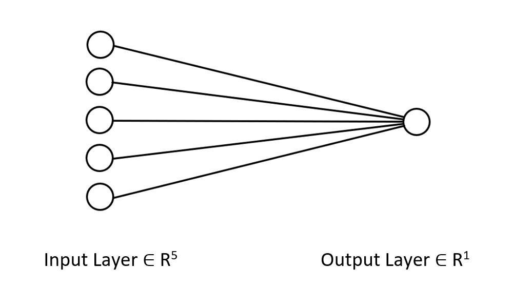
It's just a single layered neural network, that's why you see no loops in the forward pass, in the function I have just showed. Though if you follow the same matrix approach by ensuring the dimensions I just explained above, you will be able to implement architectures of any complexity.
You have seen the forward pass with the W matrix, let's see how we can generate the weights for our model.
Generating the Weights
Generating the suitable weights for the neural network is not just a matter of initializing the random values. I learned the hard way; getting this wrong will cause you all sorts of troubles in backpropagation that will cause you to doubt and start debugging your hard-coded already complex code.
Improper weight initialization can make the whole learning process tedious and time-consuming. The network can get stuck in the local minima and can be converging very slowly.
The first step is to choose the random values, I prefer going with the random state of 42.
this.W = matrix_utils.Random(0.0, 1.0,1,m_inputs, RANDOM_STATE);
Most people end up at this step, they generate the Weights and think that's all. After selecting the random variables we need to initialize our weights using either Glorot or He Initialization.
The Xavier/Glorot Initialization works best with sigmoid and tanh activation functions, while He initialization works for the RELU and its variants
He Initialization
![]()
where: n = Number of inputs to the node.
So, after the weights were initialized the weight normalization followed.
   this.W = matrix_utils.Random(0.0, 1.0,1,m_inputs, RANDOM_STATE);
   this.W = this.W * 1/sqrt(m_inputs); //He initialization
Since this neural network has one layer, there is only a single matrix for carrying the weights.
Activation Functions
Since this is a regression type of neural network, the activation functions of this network are just the variants of the regression activation function. RELU:
enum activation
  {
   AF_ELU_ = AF_ELU,
   AF_EXP_ = AF_EXP,
   AF_GELU_ = AF_GELU,
   AF_LINEAR_ = AF_LINEAR,
   AF_LRELU_ = AF_LRELU,
   AF_RELU_ = AF_RELU,
   AF_SELU_ = AF_SELU,
   AF_TRELU_ = AF_TRELU,
   AF_SOFTPLUS_ = AF_SOFTPLUS
  };
These activation functions in red and much more are there by default provided by the standard library on matrices, READ MORE.
Loss Functions
The loss functions for this regression neural network are:
enum loss
  {
    LOSS_MSE_ = LOSS_MSE,
    LOSS_MAE_ = LOSS_MAE,
    LOSS_MSLE_ = LOSS_MSLE,
    LOSS_HUBER_ = LOSS_HUBER
  };
There are more activation functions provided by the standard library, READ MORE.
Backpropagation Using Delta Rule
Delta rule is a gradient descent learning rule for updating the weights of the inputs to artificial neurons in a single-layer neural network. This is a special case of the more general backpropagation algorithm. For a neuron j with activation function g(x), the delta rule for the neuron j's ith weight Wji is given by:
![]()
where:
![]() is a small constant called learning rate
is a small constant called learning rate
![]() is the derivative of g
is the derivative of g
g(x) is the neuron's activation function
![]() is the target output
is the target output
![]() is the actual output
is the actual output
![]() is the ith input
is the ith input
That's great we now have a formula, so we just need to implement it right? WRONG!!!
The problem with this formula is that as simple as it looks it is very complex when turning it into code and requires you to code a couple of for loops, this kind of practice in neural networks will eat you alive. The proper formula that we need to have is the one that shows us the matrix operations. Let me craft that one for you:
![]()
Where;
![]() = change in weights matrix
= change in weights matrix
![]() = Derivative of the Loss function
= Derivative of the Loss function
![]() = Element-wise matrix multiplication/ Hadamard product
= Element-wise matrix multiplication/ Hadamard product
![]() = Derivative of neuron activations matrix
= Derivative of neuron activations matrix
![]() = Inputs matrix.
= Inputs matrix.
Always the L matrix has the same size as the O matrix, and the resulting matrix on the right side needs to be of the same size as the W matrix. Otherwise, you are screwed.
Let's see how this looks like when converted into code.
for (ulong iter=0; iter<m_rows; iter++)
   {
        OUTPUT = ForwardPass(m_x_matrix.Row(iter)); //forward pass
        pred = matrix_utils.MatrixToVector(OUTPUT);

        actual[0] = m_y_vector[iter];

        preds[iter] = pred[0];
        actuals[iter] = actual[0];

//---

        INPUT = matrix_utils.VectorToMatrix(m_x_matrix.Row(iter));

        vector loss_v = pred.LossGradient(actual, ENUM_LOSS_FUNCTION(L_FX));

        LOSS_DX.Col(loss_v, 0);

        OUTPUT.Derivative(OUTPUT, ENUM_ACTIVATION_FUNCTION(A_FX));

        OUTPUT = LOSS_DX * OUTPUT;

        INPUT = INPUT.Transpose();
        DX_W = OUTPUT.MatMul(INPUT);

        this.W -= (alpha * DX_W); //Weights update by gradient descent
 }
The good thing about using the matrix library provided by MQL5 instead of arrays for machine learning is that you don't have to worry calculus, I mean you don't have to worry about finding the derivatives of the loss function, derivatives of the activation function — nothing.
To train the model we need to consider two things, at least for now epochs and the learning rate denoted as alpha. If you read my previous article in this series about gradient descent you know what I'm talking about.
Epochs: a single epoch is when the entire dataset has completely cycled forward and backward through the network. In simple words, when the network has seen all the data. The larger the number of epochs the longer it takes to train a neural network, and the better it may learn.
Alpha: is the size of the steps you want the gradient descent algorithm to take when going to the global and local minimum. Alpha is usually a small value between 0.1 and 0.00001. The larger this value, the faster the network converges but, the higher the risk of skipping the local minimum.
Below is the complete code for this delta rule:
   for (ulong epoch=0; epoch<epochs && !IsStopped(); epoch++)
      {
         for (ulong iter=0; iter<m_rows; iter++)
            {
              OUTPUT = ForwardPass(m_x_matrix.Row(iter));
              pred = matrix_utils.MatrixToVector(OUTPUT);

              actual[0] = m_y_vector[iter];

              preds[iter] = pred[0];
              actuals[iter] = actual[0];

           //---

              INPUT = matrix_utils.VectorToMatrix(m_x_matrix.Row(iter));

              vector loss_v = pred.LossGradient(actual, ENUM_LOSS_FUNCTION(L_FX));

              LOSS_DX.Col(loss_v, 0);

              OUTPUT.Derivative(OUTPUT, ENUM_ACTIVATION_FUNCTION(A_FX));

              OUTPUT = LOSS_DX * OUTPUT;

              INPUT = INPUT.Transpose();
              DX_W = OUTPUT.MatMul(INPUT);

              this.W -= (alpha * DX_W);
            }

         printf("[ %d/%d ] Loss = %.8f | accuracy %.3f ",epoch+1,epochs,preds.Loss(actuals,ENUM_LOSS_FUNCTION(L_FX)),metrics.r_squared(actuals, preds));
      }
Now everything is set up. Time to train the neural network to understand just a small pattern in the dataset.
#include <MALE5\Neural Networks\selftrain NN.mqh>
#include <MALE5\matrix_utils.mqh>

CRegNeuralNets *nn;
CMatrixutils matrix_utils;
//+------------------------------------------------------------------+
//| Expert initialization function                                   |
//+------------------------------------------------------------------+
int OnInit()
  {
//---
    matrix Matrix = {
                     {1,2,3},
                     {2,3,5},
                     {3,4,7},
                     {4,5,9},
                     {5,6,11}
                   };

   matrix x_matrix; vector y_vector;

   matrix_utils.XandYSplitMatrices(Matrix,x_matrix,y_vector);

   nn = new CRegNeuralNets(x_matrix,y_vector,0.01,100, AF_RELU_, LOSS_MSE_); //Training the Network


//---
   return(INIT_SUCCEEDED);
  }
The function XandYSplitMatrices splits our matrix into x and y matrix and vector respectively.
| X Matrix | Y Vector |
|---|---|
| { {1, 2}, {2, 3}, {3, 4}, {4, 5}, {5, 6} } | {3}, {5}, {7}, {9}, {11} |
The training outputs:
CS      0       20:30:00.878    Self Trained NN EA (Apple_Inc_(AAPL.O),H1)      [1/100] Loss = 56.22401001 | accuracy -6.028
CS      0       20:30:00.879    Self Trained NN EA (Apple_Inc_(AAPL.O),H1)      [2/100] Loss = 2.81560904 | accuracy 0.648
CS      0       20:30:00.879    Self Trained NN EA (Apple_Inc_(AAPL.O),H1)      [3/100] Loss = 0.11757813 | accuracy 0.985
CS      0       20:30:00.879    Self Trained NN EA (Apple_Inc_(AAPL.O),H1)      [4/100] Loss = 0.01186759 | accuracy 0.999
CS      0       20:30:00.879    Self Trained NN EA (Apple_Inc_(AAPL.O),H1)      [5/100] Loss = 0.00127888 | accuracy 1.000
CS      0       20:30:00.879    Self Trained NN EA (Apple_Inc_(AAPL.O),H1)      [6/100] Loss = 0.00197030 | accuracy 1.000
CS      0       20:30:00.879    Self Trained NN EA (Apple_Inc_(AAPL.O),H1)      [7/100] Loss = 0.00173890 | accuracy 1.000
CS      0       20:30:00.879    Self Trained NN EA (Apple_Inc_(AAPL.O),H1)      [8/100] Loss = 0.00178597 | accuracy 1.000
CS      0       20:30:00.879    Self Trained NN EA (Apple_Inc_(AAPL.O),H1)      [9/100] Loss = 0.00177543 | accuracy 1.000
CS      0       20:30:00.879    Self Trained NN EA (Apple_Inc_(AAPL.O),H1)      [10/100] Loss = 0.00177774 | accuracy 1.000
…
…
…
CS      0       20:30:00.883    Self Trained NN EA (Apple_Inc_(AAPL.O),H1)      [100/100] Loss = 0.00177732 | accuracy 1.000
After 5 epochs only, the neural network accuracy was 100%. That's some good news because this problem is a very easy one, so I was expecting a faster learning.
Now that this neural network has been trained let me test it using new values {7,8}. You and I both know the outcome is 15.
   vector new_data = {7,8};

   Print("Test ");
   Print(new_data," pred = ",nn.ForwardPass(new_data));
Output:
CS      0       20:37:36.331    Self Trained NN EA (Apple_Inc_(AAPL.O),H1)      Test
CS      0       20:37:36.331    Self Trained NN EA (Apple_Inc_(AAPL.O),H1)      [7,8] pred = [[14.96557787153696]]
It gave us approximately 14.97. 15 is just a double that's why it came up with those additional values, but when rounded at a 1 significant figure the output will come out as 15. This is an indication that our neural network is capable of learning on itself now. Cool
Let's give this model real-world dataset and observe what it does.
I used Tesla Stock and Apple stocks as my independent variables when trying to predict the NASDAQ(NAS 100) Index. I once read an article online from CNBC that there are 6 tech stocks that make up half the value of NASDAQ, Apple and Tesla stocks being two of them. In this example, I will be using these two stocks as independent variables for training the neural network.
input string symbol_x = "Apple_Inc_(AAPL.O)";
input string symbol_x2 = "Tesco_(TSCO.L)";

input ENUM_COPY_RATES copy_rates_x = COPY_RATES_OPEN;
input int n_samples = 100;

//+------------------------------------------------------------------+
//| Expert initialization function                                   |
//+------------------------------------------------------------------+
int OnInit()
  {

   matrix x_matrix(n_samples,2); vector y_vector;

   vector x_vector;
  //---
   x_vector.CopyRates(symbol_x,PERIOD_CURRENT,copy_rates_x,0,n_samples);
   x_matrix.Col(x_vector, 0);
   x_vector.CopyRates(symbol_x2, PERIOD_CURRENT,copy_rates_x,0,n_samples);
   x_matrix.Col(x_vector, 1);

   y_vector.CopyRates(Symbol(), PERIOD_CURRENT,COPY_RATES_CLOSE,0,n_samples);

   nn = new CRegNeuralNets(x_matrix,y_vector,0.01,1000, AF_RELU_, LOSS_MSE_);
The way my broker names these symbols, which are symbol_x and symbol_x2, may be different from yours. Don't forget to change them and add those symbols to market watch before using the test EA. The y symbol is the current symbol on the chart. Make sure you attach this EA on the NASDAQ chart.
After running the script I get these output logs:
CS      0       21:29:20.698    Self Trained NN EA (NAS100,M30) [ 1/1000 ] Loss = 353809311769.08959961 | accuracy -27061631.733
CS      0       21:29:20.698    Self Trained NN EA (NAS100,M30) [ 2/1000 ] Loss = 149221473.48209998 | accuracy -11412.427
CS      0       21:29:20.699    Self Trained NN EA (NAS100,M30) [ 3/1000 ] Loss = 149221473.48209998 | accuracy -11412.427
CS      0       21:29:20.699    Self Trained NN EA (NAS100,M30) [ 4/1000 ] Loss = 149221473.48209998 | accuracy -11412.427
CS      0       21:29:20.699    Self Trained NN EA (NAS100,M30) [ 5/1000 ] Loss = 149221473.48209998 | accuracy -11412.427
CS      0       21:29:20.699    Self Trained NN EA (NAS100,M30) [ 6/1000 ] Loss = 149221473.48209998 | accuracy -11412.427
....
....
CS      0       21:29:20.886    Self Trained NN EA (NAS100,M30) [ 1000/1000 ] Loss = 149221473.48209998 | accuracy -11412.427
What?! That's what we get after all those things we did. Things like this happen most of the time in neural networks that's why having a solid understanding of NNs is very important no matter what framework and python libraries you may try, things like this happen often.
Normalizing and Scaling the Data
I can't stress how important this is, even though not all the dataset gives the best results when normalized for instance when you normalize this simple dataset we used at first to test if this NN was working fine, you will get terrible results. The network will return values just like those values or even worse I tried it.
There are many normalizing techniques. The three most widely used of them are:
Min-Max Scaler
This is a normalization technique that scales the values of a numeric feature to a fixed range of [0, 1]. Its formula is as follows:
x_norm = (x -x_min) / (x_max - x_min)
Where:
x = original feature value
x_min = is the minimum value of the feature
x_max = is the maximum value of the feature
x_norm = is the newly normalized feature value
To select the normalization technique and normalize the data you need to import the pre-processing library. Include the file is attached at the end of the article.
I decided to add the ability to normalize the data in our neural nets library.
CRegNeuralNets::CRegNeuralNets(matrix &xmatrix, vector &yvector,double alpha, uint epochs, activation ACTIVATION_FUNCTION, loss LOSS_FUNCTION, norm_technique NORM_METHOD)
You can choose a normalization technique norm_technique among these;
enum norm_technique
 {
   NORM_MIN_MAX_SCALER, //Min max scaler
   NORM_MEAN_NORM,  //Mean normalization
   NORM_STANDARDIZATION, //standardization
   NORM_NONE    //Do not normalize.
 };
After calling the class with normalization technique added to it, I was able to get a reasonable accuracy.
nn = new CRegNeuralNets(x_matrix,y_vector,0.01,1000, AF_RELU_, LOSS_MSE_,NORM_MIN_MAX_SCALER);
Output:
CS      0       22:40:56.457    Self Trained NN EA (NAS100,M30) [ 1/1000 ] Loss = 0.19379434 | accuracy -0.581
CS      0       22:40:56.457    Self Trained NN EA (NAS100,M30) [ 2/1000 ] Loss = 0.07735744 | accuracy 0.369
CS      0       22:40:56.458    Self Trained NN EA (NAS100,M30) [ 3/1000 ] Loss = 0.04761891 | accuracy 0.611
CS      0       22:40:56.458    Self Trained NN EA (NAS100,M30) [ 4/1000 ] Loss = 0.03559318 | accuracy 0.710
CS      0       22:40:56.458    Self Trained NN EA (NAS100,M30) [ 5/1000 ] Loss = 0.02937830 | accuracy 0.760
CS      0       22:40:56.458    Self Trained NN EA (NAS100,M30) [ 6/1000 ] Loss = 0.02582918 | accuracy 0.789
CS      0       22:40:56.459    Self Trained NN EA (NAS100,M30) [ 7/1000 ] Loss = 0.02372224 | accuracy 0.806
CS      0       22:40:56.459    Self Trained NN EA (NAS100,M30) [ 8/1000 ] Loss = 0.02245222 | accuracy 0.817
CS      0       22:40:56.460    Self Trained NN EA (NAS100,M30) [ 9/1000 ] Loss = 0.02168207 | accuracy 0.823
CS      0       22:40:56.460    Self Trained NN EA (NAS100,M30


CS      0       22:40:56.623    Self Trained NN EA (NAS100,M30) [ 1000/1000 ] Loss = 0.02046533 | accuracy 0.833
I also have to admit that I did not get the desired results in a 1-hour timeframe, the neural network seemed to get better accuracy on the 30 MINS chart, and I did not bother to understand what was the reason at this point.
Ok, so 82.3% accuracy on the training data. That is a good accuracy. Let's make a simple trading strategy that this network is going to use to open trades.
The current approach I have used to collect data in the OnInit function is not reliable. I will create the function to train the networks and place it on the Init function. Our network will be trained only once in a lifetime. You are not restricted to this way though.
void OnTick()
  {
//---
     if (!train_nn)
       TrainNetwork(); //Train the network only once
     train_nn = true;

  }
//+------------------------------------------------------------------+
//|                                                                  |
//+------------------------------------------------------------------+
void TrainNetwork()
 {
   matrix x_matrix(n_samples,2); vector y_vector;
   vector x_vector;

   x_vector.CopyRates(symbol_x,PERIOD_CURRENT,copy_rates_x,0,n_samples);
   x_matrix.Col(x_vector, 0);
   x_vector.CopyRates(symbol_x2, PERIOD_CURRENT,copy_rates_x,0,n_samples);
   x_matrix.Col(x_vector, 1);

   y_vector.CopyRates(Symbol(), PERIOD_CURRENT,COPY_RATES_CLOSE,0,n_samples);

   nn = new CRegNeuralNets(x_matrix,y_vector,0.01,1000, AF_RELU_, LOSS_MSE_,NORM_MIN_MAX_SCALER);
 }
Even though this Training function seems to have everything we need to take off the market, still it is not reliable. I ran a test in the Daily timeframe and came up with an accuracy of -77%, on H4 timeframes it returned an accuracy of -11234 or something like that. When increasing the data and exercising different training samples, the neural network was inconsistent with the training accuracy it was giving me.
There are many reasons to account for this one of them being that different problems require different architectures. I guess some of the market patterns on different timeframes may be too complex for this one-layered neural network, since the delta rule is for single layers neural network. We cannot fix that for now, so I will proceed with this in a timeframe where it seems to give me good output. However, there is something we can do to improve the results and tackle this inconsistent behavior a little bit. This is to split the data with a random state.
Data splitting is more important than you think
If you are coming from a python background in machine learning you might have seen the function train_test_split from sklearn.
The purpose of splitting the data into training and testing data is not only to split the data but to randomize the dataset so that it is not in its original order. Let me explain. Since neural networks and other machine learning algorithms seek to understand the patterns in the data, having data in the order it was extracted from may be bad for the models as they will also understand the patterns due to how data have been organized and arranged. This is not a smart way to let the models learn as the arrangement is not as important as the patterns that are in the variables.
void TrainNetwork()
 {
//--- collecting the data

   matrix Matrix(n_samples,3); vector y_vector;
   vector x_vector;

   x_vector.CopyRates(symbol_x,PERIOD_CURRENT,copy_rates_x,0,n_samples);
   Matrix.Col(x_vector, 0);
   x_vector.CopyRates(symbol_x2, PERIOD_CURRENT,copy_rates_x,0,n_samples);
   Matrix.Col(x_vector, 1);

   y_vector.CopyRates(Symbol(), PERIOD_CURRENT,COPY_RATES_CLOSE,0,n_samples);
   Matrix.Col(y_vector, 2);

//---

   matrix x_train, x_test; vector y_train, y_test;

   matrix_utils.TrainTestSplitMatrices(Matrix, x_train, y_train, x_test, y_test, 0.7, 42);

   nn = new CRegNeuralNets(x_train,y_train,0.01,1000, AF_RELU_, LOSS_MSE_,NORM_MIN_MAX_SCALER);

   vector test_pred = nn.ForwardPass(x_test);

   printf("Testing Accuracy =%.3f",metrics.r_squared(y_test, test_pred));
 }
After collecting the training data, the function TrainTestSplitMatrices was introduced, given the random state 42.
void TrainTestSplitMatrices(matrix &matrix_,matrix &x_train,vector &y_train,matrix &x_test, vector &y_test,double train_size=0.7,int random_state=-1)
Making Realtime Market Predictions
To make real-time predictions on the Ontick function, there has to be code to collect data and put it inside the Input vector of a neural network forward pass function.
void OnTick()
  {
//---
     if (!train_nn)
       TrainNetwork(); //Train the network only once
     train_nn = true;

     vector x1, x2;

     x1.CopyRates(symbol_x,PERIOD_CURRENT,copy_rates_x,0,1); //only the current candle
     x2.CopyRates(symbol_x2,PERIOD_CURRENT,copy_rates_x,0,1); //only the current candle

     vector inputs = {x1[0], x2[0]}; //current values of x1 and x2 instruments | Apple & Tesla

     matrix OUT = nn.ForwardPass(inputs); //Predicted Nasdaq value

     double pred = OUT[0][0];

     Comment("pred ",OUT);
 }
Now, our neural network can make predictions. Let's try to use it in trading activity. For this we will create a strategy.
Trading Logic
The trading logic is simple: If the predicted by the neural network is above the current price, open a buy trade with a take profit placed at the predicted price times a certain input value market as take profit and vice versa for sell trades. On each of the trades a stop loss is placed at some take profits point values times a certain input value marked as stop loss. Below is how things look in MetaEditor.
     stops_level = (int)SymbolInfoInteger(Symbol(),SYMBOL_TRADE_STOPS_LEVEL);
     Lots = SymbolInfoDouble(Symbol(),SYMBOL_VOLUME_MIN);
     spread = (double)SymbolInfoInteger(Symbol(), SYMBOL_SPREAD);

     MqlTick ticks;
     SymbolInfoTick(Symbol(), ticks);

     if (MathAbs(pred - ticks.ask) + spread > stops_level)
        {
          if (pred > ticks.ask && !PosExist(POSITION_TYPE_BUY))
            {
               target_gap  = pred - ticks.bid;

               m_trade.Buy(Lots, Symbol(), ticks.ask, ticks.bid - ((target_gap*stop_loss) * Point()) , ticks.bid + ((target_gap*take_profit) * Point()),"Self Train NN | Buy");
            }

          if (pred < ticks.bid && !PosExist(POSITION_TYPE_SELL))
            {
               target_gap = ticks.ask - pred;

               m_trade.Sell(Lots, Symbol(), ticks.bid, ticks.ask + ((target_gap*stop_loss) * Point()), ticks.ask - ((target_gap*take_profit) * Point()), "Self Train NN | Sell");
            }
        }
That's our logic. Let's see how the EA does on MT5.
This simple Expert Advisor can now make trades on its own. We cannot assess its performance for now; it's too soon. Let's jump to the strategy tester.
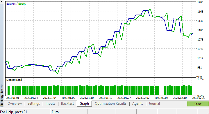
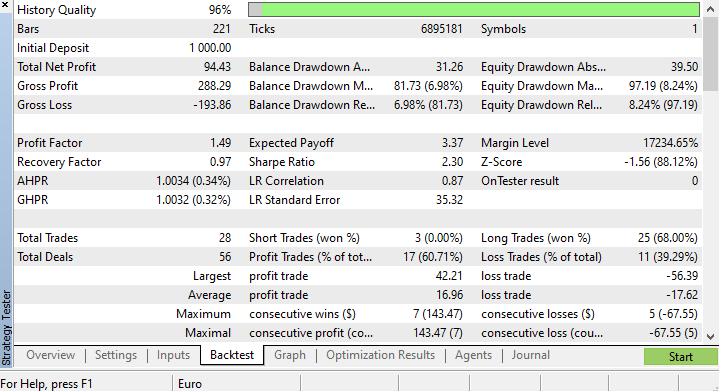
Results from the Strategy Tester
There are always challenges associated with running machine learning algorithms from the strategy tester because you have to ensure that the algorithms run smoothly and fast while ensuring that you end up in profits too.
I ran a test from 2023.01.01 to 2023.02.23 on a 4-HOUR chart based on Real ticks, I ran a test of recent ticks as I suspect it to be of much better quality compared to running on many years and months prior.
Since I set the function that trains our model to run at the very first tick of a testing life cycle, the process of training and testing the model was done instantly. Let's see how the model performed before we can see the charts and everything the strategy tester provides.
CS      0       15:50:47.676    Tester  NAS100,H4 (Pepperstone-Demo): generating based on real ticks
CS      0       15:50:47.677    Tester  NAS100,H4: testing of Experts\Advisors\Self Trained NN EA.ex5 from 2023.01.01 00:00 to 2023.02.23 00:00 started with inputs:
CS      0       15:50:47.677    Tester    symbol_x=Apple_Inc_(AAPL.O)
CS      0       15:50:47.677    Tester    symbol_x2=Tesco_(TSCO.L)
CS      0       15:50:47.677    Tester    copy_rates_x=1
CS      0       15:50:47.677    Tester    n_samples=200
CS      0       15:50:47.677    Tester    =
CS      0       15:50:47.677    Tester    slippage=100
CS      0       15:50:47.677    Tester    stop_loss=2.0
CS      0       15:50:47.677    Tester    take_profit=2.0
CS      3       15:50:49.209    Ticks   NAS100 : 2023.02.21 23:59 - real ticks absent for 2 minutes out of 1379 total minute bars within a day

CS      0       15:50:51.466    History Tesco_(TSCO.L),H4: history begins from 2022.01.04 08:00
CS      0       15:50:51.467    Self Trained NN EA (NAS100,H4)  2023.01.03 01:00:00   [ 1/1000 ] Loss = 0.14025037 | accuracy -1.524
CS      0       15:50:51.468    Self Trained NN EA (NAS100,H4)  2023.01.03 01:00:00   [ 2/1000 ] Loss = 0.05244676 | accuracy 0.056
CS      0       15:50:51.468    Self Trained NN EA (NAS100,H4)  2023.01.03 01:00:00   [ 3/1000 ] Loss = 0.04488896 | accuracy 0.192
CS      0       15:50:51.468    Self Trained NN EA (NAS100,H4)  2023.01.03 01:00:00   [ 4/1000 ] Loss = 0.04114715 | accuracy 0.259
CS      0       15:50:51.468    Self Trained NN EA (NAS100,H4)  2023.01.03 01:00:00   [ 5/1000 ] Loss = 0.03877407 | accuracy 0.302
CS      0       15:50:51.469    Self Trained NN EA (NAS100,H4)  2023.01.03 01:00:00   [ 6/1000 ] Loss = 0.03725228 | accuracy 0.329
CS      0       15:50:51.469    Self Trained NN EA (NAS100,H4)  2023.01.03 01:00:00   [ 7/1000 ] Loss = 0.03627591 | accuracy 0.347
CS      0       15:50:51.469    Self Trained NN EA (NAS100,H4)  2023.01.03 01:00:00   [ 8/1000 ] Loss = 0.03564933 | accuracy 0.358
CS      0       15:50:51.470    Self Trained NN EA (NAS100,H4)  2023.01.03 01:00:00   [ 9/1000 ] Loss = 0.03524708 | accuracy 0.366
CS      0       15:50:51.470    Self Trained NN EA (NAS100,H4)  2023.01.03 01:00:00   [ 10/1000 ] Loss = 0.03498872 | accuracy 0.370


CS      0       15:50:51.662    Self Trained NN EA (NAS100,H4)  2023.01.03 01:00:00   [ 1000/1000 ] Loss = 0.03452066 | accuracy 0.379
CS      0       15:50:51.662    Self Trained NN EA (NAS100,H4)  2023.01.03 01:00:00   Testing Accuracy =0.717
The training accuracy was 37.9% but the testing accuracy came out to be 71.7%. WHAT?!
I'm certain about what is exactly wrong, but I do suspect the training quality. Always ensure your training and testing data has a decent quality, each hole in the data could lead to a different model. Since we are looking for good results on the strategy tester too we have to be sure that the back-testing results come out of the good model that we have put a lot of energy to build.
At the end of the strategy tester, the results weren't surprising, the majority of the trades opened by this EA ended in losses of 78.27%.
Since we haven't optimized for the stop loss and take profit targets, I think it will be a good idea to optimize for these values and other parameters.
I ran a short optimization and picked up the following values. copy_rates_x: COPY_RATES_LOW, n_samples: 2950, Slippage: 1, Stop loss: 7.4, Take profit: 5.0.
This time the model gave a 61.5% training accuracy and a 63.5% testing accuracy at the beginning of the strategy tester. Seems reasonable.
CS      0       17:11:52.100    Self Trained NN EA (NAS100,H4)  2023.01.03 01:00:00   [ 1000/1000 ] Loss = 0.05890808 | accuracy 0.615
CS      0       17:11:52.101    Self Trained NN EA (NAS100,H4)  2023.01.03 01:00:00   Testing Accuracy =0.635
Final Thoughts
The Delta rule is for single-layered regression-type neural networks, keep that in mind. Despite using a single-layer neural network, we have seen how it can be built and improved when things are not going well. A single layer neural network is just a combination of linear regression models working together as a team to solve a given problem. For example:

You can look at it like 5 linear regression models working on the same issue. It's worth mentioning that this neural network is not capable of understanding complex patterns in the variables so don't be surprised if doesn't. As said earlier the Delta rule is the building block of the general backpropagation algorithm which is used for far more complex neural networks in deep learning.
The reason I built a neural network while making myself vulnerable to errors is to explain a point so that you understand that even though neural networks are capable of learning patterns you need to pay attention to small details and get a lot of things right for it to even work.
Best Regards.
Track the development of this library and many other ML models on this repo https://github.com/MegaJoctan/MALE5
Attachments table:
| File | Contents & Usage |
|---|---|
| metrics.mqh | Contains functions to measure accuracy of Neural Networks models. |
| preprocessing.mqh | Contains functions to scale and prepare the data for Neural Networks models |
| matrix_utils.mqh | Matrix manipulation additional functions |
| selftrain NN.mqh | The main include file that contains self-training neural networks |
| Self Train NN EA.mq5 | An EA for testing the self-trained neural networks |
Reference Articles:
-
Matrix Utils, Extending the Matrices and Vector Standard Library Functionality
-
Data Science and Machine Learning — Neural Network (Part 02): Feed forward NN Architectures Design
-
Data Science and Machine Learning (Part 06): Gradient Descent
Disclaimer: This article is for educational purposes only. Trading is a risky game; you should understand the risk associated with it. The author will not be responsible for any losses or damage that may be caused by using such methods discussed in this article. Risk the money you can afford to lose.