Adaptive indicators

Aleksej Poljakov | 9 December, 2022

Introduction

Probably, every trader's dream is an indicator able to adapt to the current market situation, define flat and trend segments and consider relevant price changes. Conventional technical indicators use constant ratios when handling input signals. These ratios do not depend in any way on the characteristics of the input signal and its changes over time.

Adaptive indicators are distinguished by the presence of feedback between the values of the input and output signals. This feedback allows the indicator to independently adjust to the optimal processing of financial time series values. To put it even more simple, an adaptive indicator is a regular linear indicator with its ratios being able to change over time depending on the current market situation.

Adaptation algorithms are quite diverse. Choosing a specific algorithm depends on the purpose of the indicator. But most often, these algorithms are based on various methods of least squares. Let's look at a few examples of developing an adaptive indicator.

First try

Let's try to create an adaptive indicator. The most obvious way to adapt an indicator is to take into account its latest errors in one way or another. Let's see how this can be done.

Let Indicator[i] is an indicator value on the i th bar. Then the error is Error[i] = price[i] - Indicator[i].

This error can be used to correct the indicator values during the next counting. Moreover, we can handle errors in different ways. For example, we can take the average of the last few errors, or apply exponential smoothing to them.

Let's see how this approach will look on the chart. I will use the template from the article about technical indicators as a basis. However, I will make a few changes to it. First of all, set the number of errors for

      double sum=0;
      for(int j=0; j<size; j++)
         sum=sum+coeff[j]*price[i+j];//Calculate the indicator value

      if(i>0)
        {
        double cur_error=price[i]-sum;//Current error
         if(NumErrors==0)
            cur_error=(error+cur_error)/2;
         if(NumErrors==1)
            error=cur_error/2;
         if(NumErrors>1)
           {
            for(int j=NumErrors-1; j>0; j--)
               errors[j]=errors[j-1];
            errors[0]=cur_error;

            cur_error=0;
            for(int j=0; j<NumErrors; j++)
               cur_error=cur_error+errors[j];
            error=cur_error/NumErrors;
           }
        }

      buffer[i]=sum+error;//Indicator value considering the error

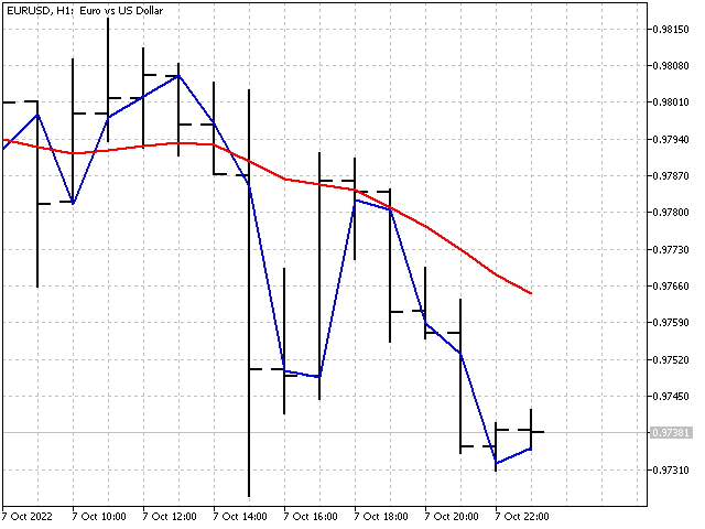
This is how our new indicator will look compared to the simple moving average (red line).

The picture looks nice, but is our indicator adaptive? Unfortunately, it is not. In fact, we have got an ordinary linear indicator, although its weight coefficients are set implicitly.

Let's take a simple moving average with the period of 3 featuring the averaging of the last three errors. Let's calculate the errors first:

Error[1] = price[1] - (price[1] + price[2] + price[3])/3

Error[2] = price[2] - (price[2] + price[3] + price[4])/3

Error[3] = price[3] - (price[3] + price[4] + price[5])/3

Then the indicator equation will look as follows:

Indicator[0] = (price[0] + price[1] + price[2])/3+(Error[1] + Error[2] + Error[3])/3 =>

Indicator[0] = (3*price[0] + 5*price[1] + 4*price[2] + 0*price[3] - 2*price[4] - 1*price[5])/9

As a result, we have got a regular linear indicator. This entails a simple conclusion – the error handling alone does not make the indicator adaptive.

Sunrise

Pierre-Simon Laplace once formulated the problem that has come to be known as "sunrise problem". The essence of this problem can be described as follows - if we saw the sunrise for 1000 days, then what will be our confidence that the sun will rise on the 1001 st day? The problem is interesting. Let's look at it from the trading perspective. Suppose that you have made nine trades, six of which turned out to be profitable. Based on this information, try to answer the question: what is the probability of a profitable trade?

As a rule, the probability is defined as the ratio of profitable trades to their total number:

In our example, the probability will be 6/9. However, we will take a step further - what is the probability of winning for a future trade? The denominator of the fraction will increase by one for any outcome. But with the numerator, two options are possible - a future transaction may turn out to be either profitable, or unprofitable. In other words, we have two possible options:

Let's take the average of these values. In this case, our estimate of the probability of winning will be as follows:

This is slightly less than the original value of 6/9. This method is called Laplace smoothing. It can be used for categorical data, where variables can take on multiple defined values ("success or failure" in our example).

Let's try to apply this smoothing in the indicator. To do this, we will make one small assumption. We will assume that there is another hidden price in the price flow (let's call it imaginary), which will also affect the indicator readings.

Let's see how the indicator equation changes in this case. This is how the simple moving average equation looks like:

And this is how the same average with an imaginary price will look like:

At first glance, everything looks great. But there are a few unpleasant things here. First, the imaginary price itself will be unstable:

Second, if we move the imaginary price to the next point in the time series, then our indicator will be simplified:

This simplification did not help us to make the indicator stable (price[1] ratio is equal to 1). However, this failure may serve as the basis for another indicator.

First, set the iPeriod indicator period. Then find the SL values for all N with the values from 1 to iPeriod. The next step is to calculate the average of the sum of all SL values. As a result, we will have an indicator showing a stable price value. This indicator can be described as follows: a naive forecast (past=future) plus a slightly weakened linear trend.

Now we have an indicator. However, adaptation has not been achieved. Another try and another fiasco. Let's take a short break, and then try to create an adaptive indicator after all. Otherwise, I will have to change the title of the article.

Moonset

A fictional Russian author Kozma Prutkov once very wisely said: "If ever asked: What's more useful, the sun or the moon, respond: the moon. For the sun only shines during daytime, when it's bright anyway, whereas the moon shines at night". Let's see how this saying can be translated into the world of trading.

In the Laplace smoothing, we used price values with the same weight ratios. But what happens if we give prices certain weights? In window functions, the weight ratios depend on how far the given reading is from the weight center of the indicator. Now we will do it differently. First, we will choose a certain price value as the central one. It will carry the most weight. The weight ratios of the rest of the prices will depend on how far the price is from this value - the farther, the less its weight will be. In other words, we will create a window function not in the time domain, but in the price domain. Let's see how such an algorithm would look in practice.

      double value=price[i+center],//Price value at the center
             max=_Point;           //Maximum deviation
      for(int j=0; j<period; j++)//Calculate price deviations from the central one and the max deviation
        {
         weight[j]=MathAbs(value-price[i+j]);
         max=MathMax(max,weight[j]);
        }

      double width=(period+1)*max/period,//correct the maximum deviation from the center so that there are no zeros at the ends
             sum=0,
             denom=0;
      for(int j=0; j<period; j++)//calculate weight ratios for each price
        {
         if(Smoothing==Linear)//linear smoothing
            weight[j]=1-weight[j]/width;
         if(Smoothing==Quadratic)//quadratic smoothing
            weight[j]=1-MathPow(weight[j]/width,2);
         if(Smoothing==Exponential)//exponential smoothing
            weight[j]=MathExp(-weight[j]/width);

         sum=sum+weight[j]*price[i+j];
         denom=denom+weight[j];
        }

      buffer[i]=sum/denom;//indicator value

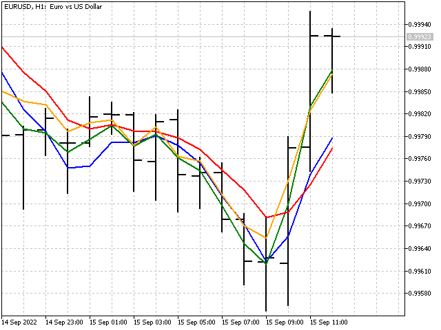
This is how our indicator looks on the chart.

The indicator weight ratios change. But we cannot call it adaptive. It would be more correct to say that this indicator adjusts to the current market situation. The adaptive indicator did not work out, but at least we took the first step.

Second try

Let's use a rectangular window function as a basis. But, let's make small changes to it - suppose that the ratios at the beginning and the end of the window can change. Then the indicator formula will look like this:

where N is an indicator period, while C1 and C2 are adaptive ratios.

Suppose that we already have the values of these ratios. A new price value appears. Along with this, the indicator error may change.

To reduce the error, we need to correct each ratio by a certain R correction factor:

It goes without saying that I will strive to ensure that changes in the ratios reduce the indicator error to zero. But this will not be the only condition. Let's additionally demand that R corrections are small as well. If both conditions are met, we can hope that the values of the adaptive ratios will fluctuate around some optimal values (if any).

So, we need to find a solution to the following problem:

Let's use the least squares method to find the R corrections. In this case, the calculations can be done in several steps. First, calculate the convergence factor:

Then, the correction values will be equal to R = price*Error*M.

Accordingly, the equations for updating the ratios will be as follows:

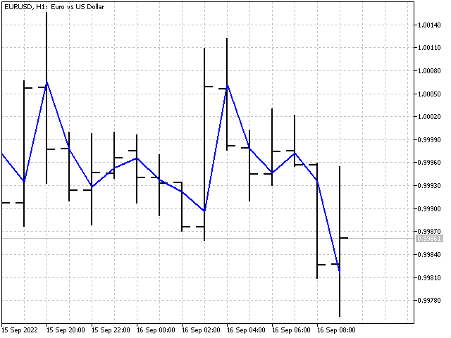
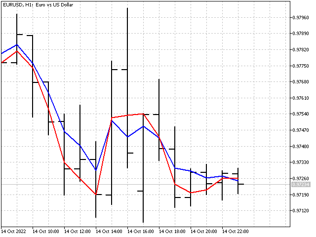
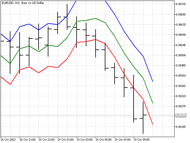
This is how our indicator will look compared to the simple moving average (red line).

Adaptation

We have managed to cope with two ratios. Is it possible to create an indicator with all its ratios being adaptive? Yes, it is. Calculations of the ratios of such an indicator are similar to those considered in the previous case. The only difference is the calculation of the convergence factor:

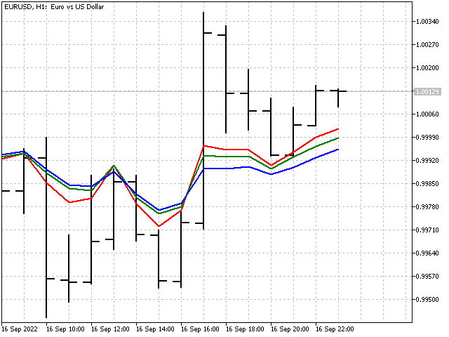
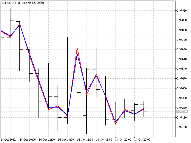
The P parameter allows adjusting the rate of change of the ratios at each step. Its value should be 1 or higher. In case of a small P, the indicator ratios reach optimal values very quickly. However, changes in the indicator ratios may turn out to be excessive. In case of a large P, the indicator ratios will change slowly. The higher the P value, the smoother the indicator will be. For example, this is what the indicators look like when P = 1 and P = 1000.

General recommendation: first set the parameter value equal to the indicator period, and then change it in one direction or another until you get the desired result.

An important feature of adaptive indicators is their potential instability. The sum of the ratios of such an indicator is not equal to one, and may vary depending on the input data. Let's take the exponential average as an example. The conventional equation looks like this: .

The adaptive EMA equation will be like this:  .

C1 and C2 do not depend on each other. The ratios are updated in the same way as in the previous indicator. The difference is in the fact that the previous values of the indicator itself are used apart from the prices.

Then, the updated ratios will be equal to:

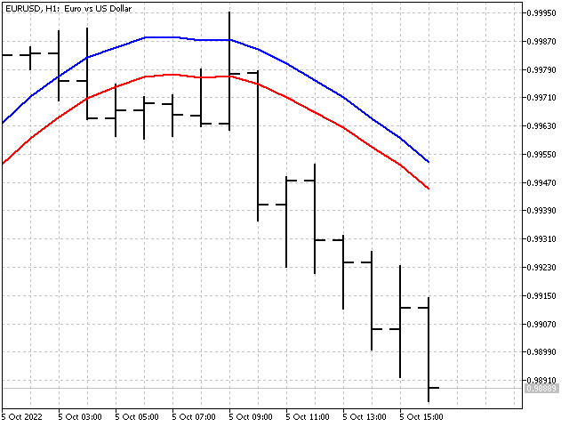
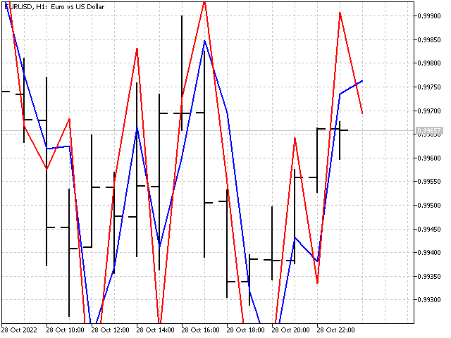
Adaptive EMA itself with different P values looks like this.

Adaptation algorithms can also be applied to window functions. However, the result will not be so impressive, since the adaptation will occur due to a change in the normalizing ratio.

Let's take the LWMA indicator with a period of 5 as a basis. Its equation can be written like this: .

Here C is a normalizing ratio. In the usual case, the value of this ratio is constant and can be calculated in advance. Now we will allow the possibility of its change in one direction or another.

First, we need to calculate the weighted sum:  .

In this case, the adjusted value of the normalizing ratio can be found using the following equation:

This approach can be useful for indicators with a short period. For long periods, the influence of adaptation and P parameter will be almost invisible.

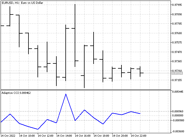
Based on adaptive indicators, we can create a variety of oscillators. For example, this is how the CCI adaptive indicator looks like.

Linear prediction

Building an adaptive indicator is in many ways similar to solving a linear prediction problem. Indeed, if we use the difference between the indicator value and the future (in relation to the indicator itself) price as an error, then the adaptive indicator will turn into a predictive one.

For example, let's take open prices. Then the indicator equation and the error value will be as follows:

All other calculations are performed according to equations that are already familiar to us. The only thing we will add to this indicator is the calculation of the average forecast error. As a result, we get the predicted value of the open price for a bar with an index of -1.

Linear probabilistic forecast

The task of linear forecasting can also be expressed in terms of the price movement equation. In the physical world, everything looks quite simple: if the current position of a point, its speed and acceleration are known, then it will not be difficult to predict its position at the next moment in time. In case of the price movement, all is more complicated.

We know the value of the price. In the language of math, velocity and acceleration are the first and second derivatives. We will replace them with a discrete analog - divided differences of the corresponding order. The ratios of the divided differences can be taken from the corresponding row of Pascal's triangle. We just need to alternately change the signs in front of each ratio. This way we will get:

1*open[0] -1*open[1] – discrete analog of speed;

1*open[0] -2*open[1] +1*open[2] – discrete analogue of acceleration.

Then the price movement equation can be expressed as follows:

open[0] + (open[0] – open[1]) + (open[0] – 2*open[1] + open[2]).

We add adaptive ratios to this equation and as a result we get:

open[-1] = open[0] + c1*(open[0] – open[1]) + c2*(open[0] – 2*open[1] + open[2]).

Let's open the brackets and arrange the ratios. Then the equation will look as follows:

open[-1] = (1 + с1 + с2)*open[0] + (-c1 – 2*с2)*open[1] + c2*open[2].

As you might remember, the ratios of a stable indicator should lie in the range from -1 to +1. Then, we need to solve the following set of inequalities:

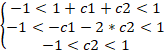
As a result, we get three possible options:

Now we can choose ratio values and use them in the indicator.

Of course, the use of higher order differences will give more possible options and will favorably affect the appearance of the indicator.

Conclusion

The use of adaptation algorithms makes it possible to obtain pretty unusual indicators. Their main advantage is self-adjustment to the current market situation. The disadvantages include an increase in the number of control parameters, the selection of which may require some time. On the other hand, adaptive indicators can change in a very wide range, which can yield new approaches to technical analysis.