Data Science and Machine Learning (Part 07): Polynomial Regression

Omega J Msigwa | 6 October, 2022

Table of contents:

Introduction

We are not through with regression models, we are back in it for a second. As I said in the first article of this series the basic linear regression serves as a foundation for many machine learning models and today we are going to discuss something a little bit different from linear regression known as Polynomial regression.

Machine Learning has changed our world a lot in many ways, we have different methods to learn the training data for classification and regression problems, such as linear regression, logistic regression, support vector machine, polynomial regression, and many other techniques, Some parametric methods like polynomial regression and support vector machines stand out as being versatile.

They create simple boundaries for simple problems and nonlinear boundaries for complex problems

Linear and non linear boundaries

Reminder of Polynomials

A polynomial is any mathematical expression that looks like this;

Polynomial equation 01:

We have our data x then it's taken to increasing high powers then we have some coefficients which are taking to scaling our data.

Here is another example of polynomial regression

Polynomial equation 02

5 corresponds to ao -7 corresponds to a1, 4 corresponds to a2, and 11.3 corresponds to a3.

In polynomial you won't necessarily need to have every single x term in here, let's see this equation;

Polynomial equation 03

You can think of it as writing

Order of Polynomials

There is another concept in polynomials called the order, The order of the polynomial is denoted by n. It is the highest coefficient in the mathematical expression for example:

Polynomial equation 01 above, is a nth order polynomial regression
Polynomial equation 02 above, is a third order/degree polynomial regression
Polynomial equation 03 above, is also a third order/degree polynomial regression

Some people get confused because in the second equation we have 3 variables multiplied by x and their coefficients are in ascending order 1,2,3 meanwhile in the second equation we only have two variables. Well, the order of the polynomial is primarily determined by the highest coefficient in the expression.

Polynomial Regression

Polynomial regression is one of the machine learning algorithms used for making predictions, I heard that it was widely used to predict the spread rate of COVID-19 and other infectious diseases, Let's see what this algorithm is made up of.
Looking at a simple linear regression model.

linear regression equation

Notice something?

This simple linear regression is nothing but a first-order polynomial regression, depending on the polynomial regression the order we can add variables to it, for instance, a second-order polynomial regression would look like this:

polynomial regression

We can get this expression to be higher in order,

kth order polynomial regression

This is the kth order polynomial regression, Wait a second is this still a linear regression? what happened to the linear model.

What happened to the linearities?

Didn't I say in the previous articles that regression is all about the linear model? How can we fit this polynomial regression to the linearities when we have these squared term coefficients. It all comes down to what needs to be linear and what can be nonlinear. The coefficients/Betas are all linear it's just the data themselves that gets raised to higher powers.

Polynomial regression vs linear regression

When should one use Polynomial regression?

We all know that the basic linear model is not good at fitting slightly complex data(nonlinear) or figuring out complex relationships in the dataset, Polynomial regression is here to solve that problem. Imagine trying to predict the price of NASDAQ using the APPLE stock price, Apple being one of the biggest influencers behind the price of NASDAQ it's relationship is still not linear so the linear model might not be able to fit our dataset to the point where we can trust it to make future predictive decisions. Let's see how the graph of these two symbols looks like on the same axis by creating a scatterplot to present the price values.

Below is the function to create a scatter plot on the terminal, thanks to CGraphics (I never knew such thing is possible until the moment I was writing this Article)

bool ScatterPlot(
                 string obj_name,
                 vector &x,
                 vector &y,
                 string legend,
                 string x_axis_label = "x-axis",
                 string y_axis_label = "y-axis", 
                 color  clr = clrDodgerBlue,
                 bool   points_fill = true                 
                )
 { 
   if (!graph.Create(0,obj_name,0,30,70,440,320))
     {
       printf("Failed to Create graphical object on the Main chart Err = %d",GetLastError());
       return(false);
     }
   
   ChartSetInteger(0,CHART_SHOW,ChartShow);
   
   double x_arr[], y_arr[]; 
   
   pol_reg.vectortoArray(x,x_arr);
   pol_reg.vectortoArray(y,y_arr);
   
   CCurve *curve = graph.CurveAdd(x_arr,y_arr,clr,CURVE_POINTS);
   curve.PointsSize(10);
   curve.PointsFill(points_fill); 
   curve.Name(legend);
   graph.XAxis().Name(x_axis_label);
   graph.XAxis().NameSize(10);
   graph.YAxis().Name(y_axis_label);
   graph.YAxis().NameSize(10);
   graph.FontSet("Lucida Console",10);
   graph.CurvePlotAll();
   graph.Update();
 
   delete(curve);
   
   return(true);
 }

   string plot_name = "x vs y"; 
   
   ObjectDelete(0,plot_name);    
   ScatterPlot(plot_name,x_v,y_v,X_symbol,X_symbol,Y_symol,clrOrange);

Output:

Nasdaq vs Apple graph

You can't deny the fact that the linear model will not perform well in this kind of problem, so let's try polynomial regression. This now, this raises the question of which order should one use to make a polynomial model?

Looking at the model expression;

polynomial regression

Since we have just one independent variable we can bring it to any power we want, Again how do we know what power should we raise this one independent variable in other words how do we know what order the polynomial should be, To understand this let's first understand something called Bayesian information criterion denoted as BIC.

Bayesian Information Criterion

its formula is given below,

BIC = n log(SSE) + k log (n)

n = number of data points

k = number of parameters

But before we figure out the best model let's create a basic Polynomial Regression and see what makes it tick, from there we can proceed on finding the best order.

Finding the Coefficients of the model.

From the equation,

second degree polynomial linear regression

Let's solve this second-degree polynomial regression task by finding the values of b0, b1, and b2.

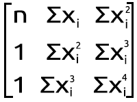
We use the following system of equations,

n = number of data points

To calculate the values, let's use this simple dataset.

X	y
3	2.5
4	3.2
5	3.8
6	6.5
7	11.5

We now have a set of simultaneous equations for our problem and the simple dataset to build things upon, you can easily plug in the values in and find the coefficients in a scientific calculator, Microsoft excel or something you'd prefer, You will get the values;

b0 = 12.4285714
b1= -5.5128571
b2 = 0.7642857

But that's not our thing here in MQL5, let's find out how to achieve this result in Meta editor from the set of the above simultaneous equation, Let's transform it into the matrix form, It now then becomes

simultaneous matrix Polynomial matrix figure

The result of this multiplication leads us back to the simultaneous equation. so you know we are mathematically correct,

Now let's write some code;

Polynomial regression class:

class CPolynomialRegression
  {
   private:
                        ulong  m_degree; //depends on independent vars
                        int    n;   //number of samples in the dataset
                        vector x;
                        vector y;
                        matrix PolyNomialsXMatrix; //x matrix 
                        matrix PolynomialsYMatrix; //y matrix 
                        matrix Betas;
                        double Betas_A[];  //coefficients of the model stored in Array

                        void   Poly_model(vector &Predictions,ulong degree);
                        
   public:
                        CPolynomialRegression(vector& x_vector,vector &y_vector,int degree=2);
                       ~CPolynomialRegression(void);
                        
                        double RSS(vector &Pred);               //sum of squared residuals
                        void   BIC(ulong k, vector &bic,int &best_degree);      //Bayessian information Criterion
                        void   PolynomialRegressionfx(ulong degree, vector &Pred);
                        double r_squared(vector &y,vector &y_predicted); 
                        
                        void   matrixtoArray(matrix &mat, double &Array[]);
                        void   vectortoArray(vector &v, double &Arr[]);
                        void   MinMaxScaler(vector &v);
  };

Our class is primarily simple and doesn't have complicated code to read, at first if any changes will be made, the code will be updated on the files attached below because I am writing this code at the time I am also writing this post.

From our matrix expression on the polynomial matrix image figure above, we can see that we have a lot of summation on each data point raised on its own exponent since this calculation is on demand for almost each and every element in our first array on the right-hand side of the equal sign, below is a short example code on how to do it.

    vector c;
    vector x_pow;
    
    for (ulong i=0; i<PolynomialsYMatrix.Rows(); i++)
       for (ulong j=0; j<PolynomialsYMatrix.Cols(); j++) 
         {
            if (i+j == 0)  PolynomialsYMatrix[i][j] = y.Sum(); 
            else         
               {
                   x_pow = MathPow(x,i);       c = y*x_pow; //x vector elements are raised to the power i then the resulting vector is  
                                                                //Then multiplied to the vector of y values the output is stored in a vector c
                   PolynomialsYMatrix[i][j] =  c.Sum();     //Finally the sum of all the elements in a vector c is stored in the matrix of polynomials
               }
         }

Looking at the Matrix in the right hand side of the Polynomial matrix image figure above you will also notice that we have function Σxy and Σxy^2 now this is a slightly different approach so let's also see the code on how to do it

  
   double pow = 0;
   ZeroMemory(x_pow);
   
    for (ulong i=0,index = 0; i<PolyNomialsXMatrix.Rows(); i++)
       for (ulong j=0; j<PolyNomialsXMatrix.Cols(); j++, index++)
          {
             pow = (double)i+j; //The power corresponds to the access index of rows and cols i+j
             if (pow == 0) PolyNomialsXMatrix[i][j] = n;
             else          
                 {
                   x_pow = MathPow(x,pow); //x_pow is a vector to store the x vector raised to a certain power
                   
                   PolyNomialsXMatrix[i][j] =  x_pow.Sum(); //find the sum of the power vector
                 }
          }

Now that we have these summations lines of codes which proves to be of much importance to polynomial regression, let's proceed by creating the Matrix that will carry these values just like the second matrix on the polynomial matrix figure image.

Starting with the matrix on the left-hand side of the equals sign.

    ulong order_size = degree+1;
    PolyNomialsXMatrix.Resize(order_size,order_size);
    
    PolynomialsYMatrix.Resize(order_size,1);
    
    vector c;
    vector x_pow;
    
    for (ulong i=0; i<PolynomialsYMatrix.Rows(); i++)
       for (ulong j=0; j<PolynomialsYMatrix.Cols(); j++) 
         {
            if (i+j == 0)  PolynomialsYMatrix[i][j] = y.Sum(); 
            else         
               {
                   x_pow = MathPow(x,i);       c = y*x_pow;
                   PolynomialsYMatrix[i][j] =  c.Sum(); 
               }
         }
    
   if (debug) Print("Polynomials y vector \n",PolynomialsYMatrix);

Just by looking at how elements inside the matrix have been arranged we know the first element only is the one that does not get multiplied to the values of x, all the rest gets multiplied to the values of x raised by the index of where they are positioned in the matrix.

Switching the array at the focal point of the equation

My first observation is that this Matrix array size is equal to the squared size of the Y matrix/ Matrix on the left side we just previous calculated, also the power to which the x items are raised is based upon where the element is positioned in the matrix by looking at rows and columns. Since this matrix is a squared one we have to build up by looping its columns twice of two respective loops, see the code below.

    ulong order_size = degree+1;
    PolyNomialsXMatrix.Resize(order_size,order_size);
    
    PolynomialsYMatrix.Resize(order_size,1);
     
    vector x_pow;
    
//---
   
   PolyNomialsXMatrix.Resize(order_size, order_size);
   
   double pow = 0;
   ZeroMemory(x_pow);
   //x_pow.Copy(x);
   
    for (ulong i=0,index = 0; i<PolyNomialsXMatrix.Rows(); i++)
       for (ulong j=0; j<PolyNomialsXMatrix.Cols(); j++, index++)
          {
             pow = (double)i+j;
             if (pow == 0) PolyNomialsXMatrix[i][j] = n;
             else          
                 {
                   x_pow = MathPow(x,pow);
                   
                   PolyNomialsXMatrix[i][j] =  x_pow.Sum();
                 }
          }
  //---

   if (debug) Print("Polynomial x matrix\n",PolyNomialsXMatrix);

Below is the output of the above code snippets.

CS      0       02:10:15.429    polynomialReg test (#SP500,D1)  Polynomials y vector 
CS      0       02:10:15.429    polynomialReg test (#SP500,D1)  [[27.5]
CS      0       02:10:15.429    polynomialReg test (#SP500,D1)   [158.8]
CS      0       02:10:15.429    polynomialReg test (#SP500,D1)   [966.2]]
CS      0       02:10:15.429    polynomialReg test (#SP500,D1)  Polynomial x matrix
CS      0       02:10:15.429    polynomialReg test (#SP500,D1)  [[5,25,135]
CS      0       02:10:15.429    polynomialReg test (#SP500,D1)   [25,135,775]
CS      0       02:10:15.429    polynomialReg test (#SP500,D1)   [135,775,4659]]

Magnificent! Now, this is where things get tricky. To find the values of the unknown Matrix of Beta values we have to look at some mathematics on matrices.

Finding the unknown values of the multiplied matrix:

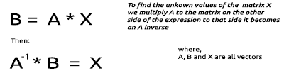
We follow the same procedure for our matrices we just obtained their values above.

finding coefficient

The process of finding the inverse of a matrix is relatively simple and takes two if not one line of code using the standard library on matrix.

    PolyNomialsXMatrix = PolyNomialsXMatrix.Inv(); //find the inverse of the matrix then assign it to the original matrix

Finally, to find the coefficients of the model we have to multiply the inversed matrix to the matrix with the y values summed up.

    Betas = PolyNomialsXMatrix.MatMul(PolynomialsYMatrix);

Now, its time we print the Betas Matrix to see what we got from this process;

CS      0       02:10:15.429    polynomialReg test (#SP500,D1)  Betas 
CS      0       02:10:15.429    polynomialReg test (#SP500,D1)  [[12.42857142857065]
CS      0       02:10:15.429    polynomialReg test (#SP500,D1)   [-5.512857142857115]
CS      0       02:10:15.429    polynomialReg test (#SP500,D1)   [0.7642857142856911]]

Great, exactly what we've been looking for, Now, that we have the coefficients of the 2nd degree polynomial regression let's proceed by building the model on those.

void CPolynomialRegression::Poly_model(vector &Predictions, ulong degree)
 {
   ulong order_size = degree+1;
   Predictions.Resize(n);
   
   matrixtoArray(Betas,Betas_A); 
   
    for (ulong i=0; i<(ulong)n; i++)
     {
      double sum = 0;
       for (ulong j=0; j<order_size; j++) 
         {
           if (j == 0) sum += Betas_A[j];
           else        sum += Betas_A[j] * MathPow(x[i],j);
         }
       Predictions[i] = sum;
     }
 }

As simple as the model's code might look, it can handle as many degrees as you want it to, at least for now. Let's plot the model predictions on the same axis of x and y values

   ObjectDelete(0,plot_name);
   plot_name = "x vs y";   
   ScatterCurvePlots(plot_name,x_v,y_v,Predictions,"Predictions","x","y",clrDeepPink);

bool ScatterCurvePlots(
                       string obj_name,
                       vector &x,
                       vector &y,
                       vector &curveVector, 
                       string legend,
                       string x_axis_label = "x-axis",
                       string y_axis_label = "y-axis", 
                       color  clr = clrDodgerBlue,
                       bool   points_fill = true                 
                      )
 {
 
   if (!graph.Create(0,obj_name,0,30,70,440,320))
     {
       printf("Failed to Create graphical object on the Main chart Err = %d",GetLastError());
       return(false);
     }
   
   ChartSetInteger(0,CHART_SHOW,ChartShow);
   
   
//--- additional curves

   double x_arr[], y_arr[]; 
   
   pol_reg.vectortoArray(x,x_arr);
   pol_reg.vectortoArray(y,y_arr);

   double curveArray[]; //curve matrix array
   
   pol_reg.vectortoArray(curveVector,curveArray);
   
   graph.CurveAdd(x_arr,y_arr,clrBlack,CURVE_POINTS,y_axis_label);
   graph.CurveAdd(x_arr,curveArray,clr,CURVE_POINTS_AND_LINES,legend);
    
//---

   graph.XAxis().Name(x_axis_label);
   graph.XAxis().NameSize(10);
   graph.YAxis().Name(y_axis_label);
   graph.YAxis().NameSize(10);
   graph.FontSet("Lucida Console",10);
   graph.CurvePlotAll();
   graph.Update();
   
   return(true);
 }

Output:

It is undeniable that the polynomial model was able to fit our data well and may outperform a linear model at fitting the data in this case.

Finding the Best Polynomial Degree

As said earlier that Bayesian Information Criterion is the algorithm we use to find the best model, Let's convert the formula into code. According to BIC the model with the lowest value of BIC is the best model because that model is the one with the least sum of residuals/errors.

void  CPolynomialRegression::BIC(ulong k, vector &bic,int &best_degree)
 {
   vector Pred;
   
   bic.Resize(k-2); 
   best_degree = 0;
   
    for (ulong i=2, counter = 0; i<k; i++)
      {         
         PolynomialRegressionfx(i,Pred);         
         bic[counter] = ( n * log(RSS(Pred)) ) + (i * log(n));  
         
         counter++;
      }
      
//--- 

   bool positive = false;
   for (ulong i=0; i<bic.Size(); i++)
      if (bic[i] > 0) { positive = true; break; }
   
  
   double low_bic = DBL_MAX;
   
   if (positive == true) 
    for (ulong i=0; i<bic.Size(); i++) 
     {
      if (bic[i] < low_bic && bic[i] > 0) low_bic = bic[i];
     }
   else  low_bic = bic.Min(); //bic[ best_degree = ArrayMinimum(bic) ];
      
   printf("Best Polynomial Degree(s) is = %d with BIC = %.5f",best_degree = best_degree+2,low_bic);

 }

From the code the function RSS is Residual Sum of Squares. This function finds the sum of squared residuals.

double CPolynomialRegression::RSS(vector &Pred)
 {
  if (Pred.Size() != y.Size()) Print(__FUNCTION__," Predictions Array and Y matrix doesn't have the same size");
 
   double sum =0;
    for (int i=0; i<(int)y.Size(); i++)
      sum += MathPow(y[i] - Pred[i],2);
      
    return(sum);
 }

Now let me run this function to find the best polynomial among the 10 degrees.

   vector bic_; //A vector to store the model BIC values for visualization purposes only
   
   int best_order; //A variable to store the best model order 
   
   pol_reg.BIC(polynomia_degrees,bic_,best_order);

Below is the output when plotted on the terminal;

According to our code the best model has the polynomial degree of 2. It's undeniable that the model with the degree of 2, is the best one for this simple dataset.

2022.09.22 20:58:21.540 polynomialReg test (#NQ100,D1)  Best Polynomial Degree(s) is = 2 with BIC = 0.93358

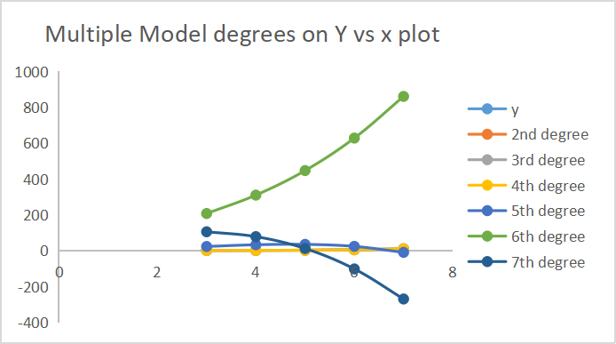
Below is the output of how each model made predictions.

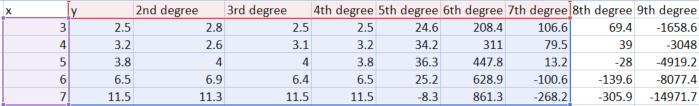
7 of the degree outputs are plotted on the same axis.

Feature Scaling is Essential

Since in polynomial regression we have only one independent variable that we can raise to any power we want scaling the feature in the first place becomes very important because if your independent variable has features in the range of 100-1000 on the second degree of these features will range between 10000 - 1000,000 in the third degree they will range between 10^6 - 10^9. OMG, that's a lot.

There are many ways and algorithms to scale the dataset but we are going to use the Min-max scaler function to scale the vectors, Keep in mind that this process should be done before any manipulations to the dataset. Below is the code for the function that will be used to scale the vectors from the dataset.

void MinMaxScaler(vector &v)
 {
   //Normalizing vector using Min-max scaler
   
   double min, max, mean;
   min = v.Min();
   max = v.Max();
   mean = v.Mean();
   
   for (int i=0; i<(int)v.Size(); i++)
     v[i] = (v[i] - min) / (max - min);  
   
 }

We now have everything we need, its time to build the model on the live market data refer to Nasdaq vs Apple graph from above. To be able to obtain the results there are several few steps we need to take.

Extracting market price data and scaling.

   if (!SymbolSelect(X_symbol,true))   printf("%s not found on Market watch Err = %d",X_symbol,GetLastError());  
   if (!SymbolSelect(Y_symol,true))    printf("%s not found on Market watch Err = %d",Y_symol,GetLastError());  
  
   matrix rates(bars, 2);
   vector price_close;

//---

   vector x_v, y_v;

   price_close.CopyRates(X_symbol,PERIOD_H1,COPY_RATES_CLOSE,1,bars); //extracting prices
   
   rates.Col(price_close,0);
   
   x_v.Copy(price_close);

//---
   
   price_close.CopyRates(Y_symol,PERIOD_H1,COPY_RATES_CLOSE,1,bars);
   
   y_v.Copy(price_close);
    
   rates.Col(price_close,1);
   
//---

   MinMaxScaler(x_v); //scalling all the close prices
   MinMaxScaler(y_v); //scalling all the close prices

//---

Below is the output presented on a scatterplot;

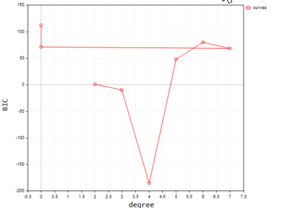
02: Finding the Best Model using the Bic Function

//--- FINDING BEST MODEL USING BIC
   
   vector bic_; //A vector to store the model BIC values for visualization purposes only
   
   int best_order; //A variable to store the best model order 
   
   pol_reg.BIC(polynomia_degrees,bic_,best_order);
   
   ulong bic_cols = polynomia_degrees-2; //2 is the first in the polynomial order 
   
//--- Plot BIc vs model degrees

   vector x_bic;
   x_bic.Resize(bic_cols);  
   for (ulong i=2,counter =0; i<bic_cols; i++)  {   x_bic[counter] = (double)i;   counter++;   }     
    
   ObjectDelete(0,plot_name);
   plot_name = "curves";
   ScatterCurvePlots(plot_name,x_bic,y_v,bic_,"curves","degree","BIC",clrBlue);
   Sleep(10000);

Below is the output

Lastly

We now know the best model order is 2. Let's make a model with 2 degrees then using it to predict the values and finally we plot the values on the graph.

   vector Predictions;
   pol_reg.PolynomialRegressionfx(best_order,Predictions); //Create model with the best order then use it to predict
   
   ObjectDelete(0,plot_name);
   plot_name = "Actual vs predictions";   
   ScatterCurvePlots(plot_name,x_v,y_v,Predictions,string(best_order)+"degree Predictons",X_symbol,Y_symol,clrDeepPink);

The resulting plot is shown below

Checking the Model Accuracy

Despite finding the best degree for the model we still need to know how that model is able to understand the relationship in our dataset by checking its predictive accuracy.

   Print("Model Accuracy = ",DoubleToString(pol_reg.r_squared(y,Predictions)*100,2),"%");

Output,

2022.09.30 16:19:31.735 polynomialReg test (#SP500,D1)  Model Accuracy = 2.36%

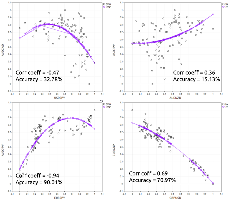
Bad news for us we got ourselves the bad model among the worst models. Now before deciding to use a polynomial regression to solve a particular task just remember that polynomial regression has linear model as the foundation of it so always have the data that is correlated, It doesn't have to be linear correlated but about 50% correlation might be ideal, looking back at our NASDAQ vs APPLE dataset and checking for it's correlation I got a correlation coefficient of less that 1%. This is probably the reason we weren't able to get a good model out of this dataset.

   Print("correlation coefficient ",x_v.CorrCoef(y_v));

To Demonstrate this point well, let's try the script on different forex instruments.

Pros and Cons of Polynomial Regression

Pros:

You can model a nonlinear relationship between the variables
There is a wide range of functions that you can use for fitting
Good for exploratory purposes. You can test different polynomial orders/degrees to see which works best for the dataset you have
It is simple to code and interpret the results yet powerful

Cons:

Outliers can seriously mess up the results
Polynomial Regression models are prone to overfitting(do doubt about that)
As a consequence of overfitting, the model may not work with the outside data

Final Thoughts

Polynomial regression is a useful Machine learning technique in many cases since the relationship between an independent variable and dependent variables isn't supposed to be linear it gives you more freedom when working with different datasets, and it helps fill the gap that the linear model can't, this technique is a better choice when the linear model is underfitting the data. That being said it is crucial that you become aware of overfitting because since this parametric model is very flexible it may perform very badly on the untrained data/testing data, I would say choose the lowest model orders and give the model room for mistakes.

Thanks for reading.

More info about matrices in array form read >> Matrices and Vectors

Further Reading | Books | References

Articles References: