Neural networks made easy (Part 29): Advantage Actor-Critic algorithm
Dmitriy Gizlyk | 25 November, 2022
Contents
- Introduction
- 1. Advantages of previously discussed reinforcement learning methods
- 2. Advantage actor-critic algorithm
- 3. Implementation
- 4. Testing
- Conclusion
- List of references
- Programs used in the article
Introduction
We continue to explore reinforcement learning methods. In previous articles we discussed methods for approximating the Q-learning Reward function and the policy gradient function learning. Each method has its own advantages and disadvantages. It would be great to use the maximum of their advantages when building and training models. When trying to find methods minimizing the shortcomings of the algorithms used, we often try to build certain conglomerates from various known algorithms and methods. In this article, we will talk about a way of combining the above two algorithms into a single model training method, which is called Advantage Actor-Critic algorithm).
1. Advantages of previously discussed reinforcement learning methods
But before we proceed to combining the algorithms, let's get back to their distinctive features, strengths and weaknesses.
When interacting with the Environment, the Agent performs some action affecting the Environment. As a result of the influence of external factors and the Agent's actions, the Environment state changes. After every state change, the Environment informs the Agent by providing some reward. This reward can be either positive or negative. The size and sign of the reward indicates the usefulness of the new state for the Agent. The Agent does not know how the reward is formed. The purpose of the Agent is to learn to perform such actions so that in the process of interaction with the Environment it can get the highest possible reward.
We first studied the algorithm for approximating the reward function Q-learning. We trained the model to learn how to predict the upcoming reward after a certain action is performed in a certain state of the environment. After that, the agent performs an action based on the predicted reward and the agent's behavior policy. As a rule, the greedy or ɛ-greedy strategy is used here. According to the greedy strategy, we choose the action with the highest predicted reward. It is most often used in the practical operation of the Agent.
The second ɛ-greedy strategy is similar to the greedy one not only in the name. It also involves choosing the action with the highest predicted reward. But it allows a random action with probability ɛ. It is used at the model training stage to better study the environment. Otherwise, having once received a positive reward, the model will constantly repeat the same action, without exploring other options. In this case, it will never know how optimal the action was or if there are any actions that could lead to a higher reward. But we want the agent to explore the environment as much as possible and get the most of it.
The advantages of the Q-learning method are obvious. The model is trained to predict rewards. It is the reward we receive from the environment. So, we have a direct relationship between the values of the model operation results and the reference values received from the environment. In this interpretation, learning is similar to supervised learning methods. When training the model, we used the standard error as a loss function.
Here you should pay attention to the following. The trained model will return the average cumulative reward until the end of the session, taking into account the discount factor that the agent received from the environment after performing a specific action in a similar state of the environment when training the model. But the environment returns a reward for each specific transition to a new state. Here we see the gap, which is covered after the Agent completes the episode.
The disadvantages of the algorithm include the complexity of model training. Previous time we had to use some tricks to train the model. First of all, successive states of the environment strongly correlate with each other. Most often they only differ only in minor detail. Direct training using such data will lead to constant retraining of the model to fit the current state. Thus, the model loses the ability to generalize data. Therefore, we had to create a buffer of historical data on which the model was trained. When training the model, we were randomly choosing states from the historical data buffer, which enabled the reduction of correlation between two states used successively in training.
By training the model on the actual data of the reward received from the environment, we get a model with low data variance. The spread of values returned by the model for each state is acceptably small. This is a positive factor. But the environment returns the reward for each specific transition. However, we want to maximize profits for the entire period. To calculate it, the Agent must complete the entire session. By using a historical data buffer and by adding a model for predicting future rewards we managed to build an algorithm that can additionally train the model in the process of its practical use. So, the learning process is running in the "on-line" mode. But we had to pay for this with an error in predicting the rewards.
While using the second model to predict future rewards, we were fully aware of errors in such predictions and accepted the risk. But each error was taken into account when training the model and influenced all subsequent predictions. Thus, we obtained a model that is able to predict results with a small variance but a large bias. This can be neglected when using a greedy strategy. During it, to choose the maximum reward, we only compare it with other rewards. Bias or scaling of values in this case does not affect the final result of the action selection.

When using Q-learning, the model is only trained to predict rewards. To select the actions, we need to specify the agent's behavior policy (strategy) at the model creation stage. But the use of the greedy strategy allows you to work successfully only in deterministic environments. This is completely inapplicable when building stochastic strategies.
The use of the policy gradient, on the contrary, does not require to determine agent's behavior policy (strategy) at the model creation stage. This method enables the agent to build its behavior policy. It can be either greedy or stochastic.
Model trained by the policy gradient method, returns the probability distribution of achieving the desired result when choosing one or another action in each specific state of the environment.
When training the model, we also use the rewards received from the environment. To select the optimal strategy in each state of the environment, a cumulative reward until the end of the session is used. Obviously, to update the weights of the model, the agent needs to go through the entire session. Perhaps this is the main disadvantage of this method. We cannot build an on-line training model because we do not know the future rewards.
At the same time, the use of the actual cumulative reward minimizes the constant error of the bias of the predicted data from their real value. This was the problem with Q-learning due to the use of predicted values of future rewards.
However, in policy gradient we train the model to predict not the expected reward but the probability distribution of achieving the desired result when the agent performs a certain action in a certain state of the environment. As the loss function, we use the logarithmic function.

To analytically determine the error minimization direction, we use the derivative of the loss function. In this case, the convenience is in the property of the logarithm derivative.

By multiplying the derivative of the loss function by the positive reward, we increase the probability of choosing such an action. And when multiplying the derivative of the loss function by a negative reward, we adjust our weights in the opposite direction. This reduces the probability of selecting this action. And reward value modulo will determine the step to adjust the weights.
As you can see, when updating the weight matrix of the model, the rewards are used indirectly. Therefore, we get a model whose results have a small bias relative to the real data, but a rather large variance of values.

The positive aspects of the method include its ability to explore the environment. When using Q-learning and ɛ-greedy strategy, we determined the balance of research to exploitation using ɛ, while the policy gradient uses sampling of actions from a given distribution.
At the beginning of training, the probabilities of performing all actions are almost equal. And the model studies the environment to the maximum, choosing one or another action of the agent with equal probability. In the process of model training, the probabilistic distribution of actions changes. The probability of choosing profitable actions increases, and it decreases for unprofitable ones. This reduces the tendency of the model to explore. The balance shifts towards exploitation.
Pay attention to one more point. Using the cumulative reward, we focus on achieving a result at the end of the session. Ans we do not evaluate the impact of each specific step. Such an approach, for example, can train the agent to hold unprofitable positions waiting for a trend reversal. Or the agent can learn to perform a large number of losing trades, the loss from which will be covered by rare profitable trades which generate high profits. Because the model will receive the final profit at the end of the session and will consider it a positive result, so the probability of such operations will increase. Of course, a large number of iterations should minimize this factor, since the ability of the method to explore the environment should help the model find the optimal strategy. But this leads to a long model training process.
Let's summarize. Q-learning models have low variance but high bias. Policy gradient, on the contrary, allows training the model with a small bias and a large variance. What we need is to be able to train the model with minimal variance and bias.
Policy gradient builds a holistic strategy without taking into account the impact of each individual step. We need to receive the maximum profit at each step, which is possible with Q-learning. Think of the Bellman function. It assumes the selection of the best action at each step.
The use of Q-function approximation methods requires the definition of the agent's behavior policy at the model creation stage. But we want the model to determine the strategy on its own based on the experience of interaction with the environment. And, of course, we wouldn't like to be limited to deterministic behavioral strategies. This can be implemented by policy training methods.
Obviously, the solution is to combine two training methods to achieve the best results.
2. Advantage actor-critic algorithm
The most successful attempts to combine reward function approximation and policy learning methods are the methods of the Actor-Critic family. Let us today get acquainted with the algorithm referred to as Advantage Actor-Critic.
The Actor-Critic family of methods involves the use of two models. One of the models, the Actor, is responsible for choosing the agent's action and is trained using policy function approximation methods. The second model, the Critic, is trained by Q-learning methods and evaluates the actions chosen by the Actor.
The first thing to do is to reduce data variance in the policy model. Let's take another look at the loss function of our policy model. Every time we multiply the logarithm of the predicted probability of the selected action by the size of the cumulative reward, taking into account discounting. The value of the predicted probability is normalized in the range [0, 1].
![]()
To reduce the variance, we can reduce the value of the cumulative reward. But it should not disturb the influence of actions on the overall result. And at the same time, it is necessary to observe data comparability for different agent training sessions. For example, we can always subtract some fixed constant or the average reward for the entire sessions.
![]()
Next, we can train the model to evaluate the contribution of each individual action. The seemingly simple idea of removing the cumulative reward and using only the reward for the current transition for training can have an unpleasant effect. First of all, getting a big reward at the current step does not guarantee us the same big reward in the future. We can get a big reward for transiting into an unfavorable state. It can be compared to "cheese in a mousetrap".
On the other hand, the reward does not always depend on the action. Most often the reward depends more on the state of the environment than on the agent's ability to evaluate this state. For example, when making deals in the direction of the global trend, the Agent can wait out corrections against the trend and wait for the price to move in the right direction. For this, the Agent does not need to analyze the current state in detail to identify trends. It is enough to correctly determine the global trend. In this case, there is a high probability of entering a position not at the best price. With a detailed analysis, it could wait for the correction and enter at a better price. But the risk of losses is much higher if correction develops into a trend change. In this case, the open position will generate big losses as there will be no reversal.
Therefore, it would be useful to compare the cumulative reward with a certain benchmark result. But how to access this value? This is where we use the Critic. We will use it to evaluate the work of the Actor.
The idea is that the Critic model is trained to evaluate the current state of the environment. This is the potential reward that the Actor can receive from the current state before the end of the session. At the same time, the Actor learns to select actions that will potentially yield greater than average rewards from previous training sessions. Thus, we replace the constant in the loss function formula above with the state estimate.
![]()
where V(s) is the environment state assessment function.
To train the state estimation function, we again use the root mean square error.
![]()
Actually, there are various approaches to building a model using this algorithm. We use two separate neural networks: one for the Actor and the other one for the Critic. But often an architecture of one neural network with two outputs is used. It is the so-called "two-headed" neural network. Part of the neural layers in this network is shared — they are responsible for processing the initial data. Several decision layers are divided into directions. Some of them are responsible for the model policy (the Actor). Others are responsible for evaluating the state (the Critic). Both the Actor and the Critic work with the same state of the environment. Therefore, they can have the same state recognition function.
There are also implementations of the on-line training of Advantage Actor-Critic models. Similar to Q-learning, the cumulative reward in them is replaced by the sum of the reward received at the last transition, and the subsequent state is evaluated taking into account the discount factor. In this case, the loss functions look like this:
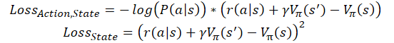
where ɣ is the discount factor.
But the on-line training has its cost. Such a model has a larger error and is more difficult to train.
3. Implementation
Now that we have considered the theoretical aspects of the method, we can proceed to the practical part of this article and build the model training process using MQL5 tools. To implement the described algorithm, we will not require any cardinal changes in the architecture of our models. We will not build a two-headed model. We will build two neural networks, Actor and Critic, using the existing means.
In addition, we will not perform the complete training of the new models. Instead, we will use two models from the last two articles. The model from the article about the Q-learning will be used as the Critic. And the model from the policy gradient article will serve as the Actor.
Please mind minor deviations from the theoretical material presented above. The Actor Model fully complies with the requirements of the considered algorithm. But the Critic Model we use slightly differs from the environment state estimation function described above. The assessment of the environment state does not depend on the action performed by the agent. The value of a state is the maximum benefit our Agent can get from this state. According to the Q-function we trained earlier, the cost of the state will be equal to the maximum value from the vector of results of this function. However, for the correct model training, we will have to take into account the action performed by the Agent in the analyzed state.
Now let us look at the method implementation code. To train the model, let us create an EA called Actor_Critic.mq5. The EA uses a template from previous articles. So, we will use two pre-trained models. The models were trained separately and were saved in different files. Therefore, first we will define files to load the models. Their names reflect a reference to the earlier articles.
#define ACTOR           Symb.Name()+"_"+EnumToString((ENUM_TIMEFRAMES)Period())+"_REINFORCE"
#define CRITIC          Symb.Name()+"_"+EnumToString((ENUM_TIMEFRAMES)Period())+"_Q-learning"
For two models, we need two instances of the neural network class. To keep the code clear, let us use the names corresponding to the models' roles in the algorithm.
CNet                Actor;
CNet                Critic;
In the EA initialization method, load the models and immediately compare the sizes of the layers of the initial data and the results. When loading the models, we cannot evaluate the comparability of models to train them on comparable samples. But we must check the comparability of model architectures. In particular, we check the size of the source data layer. Thus, we can be sure that both models use the same state description pattern to evaluate the environment state.
Then we check the results layer sizes of both models, which will allow us to compare the discreteness of the agents' possible actions.
//+------------------------------------------------------------------+
//| Expert initialization function                                   |
//+------------------------------------------------------------------+
int OnInit()
  {
//---
................
................
................
//---
   float temp1, temp2;
   if(!Actor.Load(ACTOR + ".nnw", dError, temp1, temp2, dtStudied, false) ||
      !Critic.Load(CRITIC + ".nnw", dError, temp1, temp2, dtStudied, false))
      return INIT_FAILED;
//---
   if(!Actor.GetLayerOutput(0, TempData))
      return INIT_FAILED;
   HistoryBars = TempData.Total() / 12;
   Actor.getResults(TempData);
   if(TempData.Total() != Actions)
      return INIT_PARAMETERS_INCORRECT;
   if(!vActions.Resize(SessionSize) ||
      !vRewards.Resize(SessionSize) ||
      !vProbs.Resize(SessionSize))
      return INIT_FAILED;
//---
   if(!Critic.GetLayerOutput(0, TempData))
      return INIT_FAILED;
   if(HistoryBars != TempData.Total() / 12)
      return INIT_PARAMETERS_INCORRECT;
   Critic.getResults(TempData);
   if(TempData.Total() != Actions)
      return INIT_PARAMETERS_INCORRECT;
//---
................
................
................
//---
   return(INIT_SUCCEEDED);
  }
Do not forget to control the process of how the operations are performed and save the necessary data in the appropriate variables. In particular, save the number of candlesticks of one analyzed pattern, which corresponds to the size of the initial data layer of the loaded models.
The training algorithm is implemented in the Train function. At the beginning of the function, we, as always, determine the range of the training sample.
void Train(void)
  {
//---
   MqlDateTime start_time;
   TimeCurrent(start_time);
   start_time.year -= StudyPeriod;
   if(start_time.year <= 0)
      start_time.year = 1900;
   datetime st_time = StructToTime(start_time);
Loading historical data. Make sure to check the operation execution result.
   int bars = CopyRates(Symb.Name(), TimeFrame, st_time, TimeCurrent(), Rates);
   if(!RSI.BufferResize(bars) || !CCI.BufferResize(bars) || !ATR.BufferResize(bars) || !MACD.BufferResize(bars))
     {
      ExpertRemove();
      return;
     }
   if(!ArraySetAsSeries(Rates, true))
     {
      ExpertRemove();
      return;
     }
//---
   RSI.Refresh();
   CCI.Refresh();
   ATR.Refresh();
   MACD.Refresh();
Evaluate the amount of loaded data and prepare local variables.
   int total = bars - (int)(HistoryBars + SessionSize+2);
//---
   CBufferFloat* State;
   float loss = 0;
   uint count = 0;
Next, organize a system of model training loops. The outer loop counts the number of training epochs. So, in the loop body, we define the session start point. It is selected randomly from the loaded historical data. When choosing this point, 2 factors are taken into account. First, the session start point must be preceded by historical data sufficient to form one pattern. Second, from the session start point to the end of the training sample, there should be enough historical data to complete the session.
   for(int iter = 0; (iter < Iterations && !IsStopped()); iter ++)
     {
      int error_code;
      int shift = (int)(fmin(fabs(Math::MathRandomNormal(0, 1, error_code)), 1) * (total) + SessionSize);
I did not implement the on-line learning algorithm, since we are training the model on historical data. The use of a full session usually gives better results. But at the same time, the work in the market is endless. Therefore, we have a batch implementation of the algorithm. The session size is limited by the data update batch size. This value is specified by the user in the external parameter SessionSize.
Next, create a nested loop for the initial iteration of the session. In the body of this loop, first create an object to record the parameters of the system state description. Do not forget to check the new object creation result.
      States.Clear();
      for(int batch = 0; batch < SessionSize; batch++)
        {
         int i = shift - batch;
         State = new CBufferFloat();
         if(!State)
           {
            ExpertRemove();
            return;
           }
After that, save the parameters of the current environment state. Thus we prepare a pattern for analysis at the current step of the algorithm.
         int r = i + (int)HistoryBars;
         if(r > bars)
           {
            delete State;
            continue;
           }
         for(int b = 0; b < (int)HistoryBars; b++)
           {
            int bar_t = r - b;
            float open = (float)Rates[bar_t].open;
            TimeToStruct(Rates[bar_t].time, sTime);
            float rsi = (float)RSI.Main(bar_t);
            float cci = (float)CCI.Main(bar_t);
            float atr = (float)ATR.Main(bar_t);
            float macd = (float)MACD.Main(bar_t);
            float sign = (float)MACD.Signal(bar_t);
            if(rsi == EMPTY_VALUE || cci == EMPTY_VALUE || atr == EMPTY_VALUE || macd == EMPTY_VALUE || sign == EMPTY_VALUE)
              {
               delete State;
               continue;
              }
            //---
            if(!State.Add((float)Rates[bar_t].close - open) || !State.Add((float)Rates[bar_t].high - open) ||
               !State.Add((float)Rates[bar_t].low - open) || !State.Add((float)Rates[bar_t].tick_volume / 1000.0f) ||
               !State.Add(sTime.hour) || !State.Add(sTime.day_of_week) || !State.Add(sTime.mon) ||
               !State.Add(rsi) || !State.Add(cci) || !State.Add(atr) || !State.Add(macd) || !State.Add(sign))
              {
               delete State;
               break;
              }
           }
Check the completeness of the saved data and call the feed forward pass method of the policy model.
         if(IsStopped())
           {
            delete State;
            ExpertRemove();
            return;
           }
         if(State.Total() < (int)HistoryBars * 12)
           {
            delete State;
            continue;
           }
         if(!Actor.feedForward(GetPointer(State), 12, true))
           {
            delete State;
            ExpertRemove();
            return;
           }
Then sample the agent's action from the resulting distribution.
         Actor.getResults(TempData);
         int action = GetAction(TempData);
         if(action < 0)
           {
            delete State;
            ExpertRemove();
            return;
           }
Determine the reward for the selected action. The policy reward has not changed since the last experiments in the last article. Thus, I plan to get comparable test results of the method. This will allow us to compare the impact of changes in the learning algorithm on the final result of the model, in comparison with previous tests.
         double reward = Rates[i - 1].close - Rates[i - 1].open;
         switch(action)
           {
            case 0:
               if(reward < 0)
                  reward *= -20;
               else
                  reward *= 1;
               break;
            case 1:
               if(reward > 0)
                  reward *= -20;
               else
                  reward *= -1;
               break;
            default:
               if(batch == 0)
                  reward = -fabs(reward);
               else
                 {
                  switch((int)vActions[batch - 1])
                    {
                     case 0:
                        reward *= -1;
                        break;
                     case 1:
                        break;
                     default:
                        reward = -fabs(reward);
                        break;
                    }
                 }
               break;
           }
Save the obtained values into buffers to use them later to update the model weights.
         if(!States.Add(State))
           {
            delete State;
            ExpertRemove();
            return;
           }
         vActions[batch] = (float)action;
         vRewards[SessionSize - batch - 1] = (float)reward;
         vProbs[SessionSize - batch - 1] = TempData.At(action);
         //---
        }
This concludes the iterations of the first nested loop in which information about the session is collected. After iterating through all session states, we will get a complete set of data for updating models.
Next, calculate the cumulative discounted reward for each state of the environment.
      vectorf rewards = vectorf::Full(SessionSize, 1);
      rewards = MathAbs(rewards.CumSum() - SessionSize);
      rewards = (vRewards * MathPow(vectorf::Full(SessionSize, DiscountFactor), rewards)).CumSum();
      rewards = rewards / fmax(rewards.Max(), fabs(rewards.Min()));
Now, let's calculate the value of the loss function and save the model when the best results are achieved.
      loss = (fmin(count, 9) * loss + (rewards * MathLog(vProbs) * (-1)).Sum() / SessionSize) / fmin(count + 1, 10);
      count++;
      float total_reward = vRewards.Sum();
      if(BestLoss >= loss)
        {
         if(!Actor.Save(ACTOR + ".nnw", loss, 0, 0, Rates[shift - SessionSize].time, false) ||
            !Critic.Save(CRITIC + ".nnw", Critic.getRecentAverageError(), 0, 0, Rates[shift - SessionSize].time, false))
            return;
         BestLoss = loss;
        }
Please note that we save the models before updating the weight matrices. Because these are the parameters with which the model achieved the results that we estimated by the loss function. After updating the matrices, the model will receive updated parameters and we will see the results of new parameters only after the next session completes.
At the end of the iterations of the learning epoch, we implement another nested loop in which we organize the updating of the model parameters. Here we will fetch the environment states from the buffer and pass through both models with the state removed. Remember to control the execution of operations.
      for(int batch = SessionSize - 1; batch >= 0; batch--)
        {
         State = States.At(batch);
         if(!Actor.feedForward(State) ||
            !Critic.feedForward(State))
           {
            ExpertRemove();
            return;
           }
Please note that the implementation of the feed forward pass for each model is mandatory. Even if we saved all the necessary data in the buffers. The fact is that during the back-propagation pass, the learning algorithm uses intermediate data from the calculations of neural layers. To correctly distribute the error gradient and update the weights, we need a clear arrangement of the complete chain of all intermediate values of the model for each state.
Then, update the Critic parameter. Pay attention that the model update only applies to the action selected by the Agent. The gradient of the remaining actions is considered to be zero. This difference from the previously described theoretical material is caused by the use of the pre-trained Q-function, which returns the predicted reward depending on the action chosen by the Agent. The training of the state estimation function, proposed by the authors of the method, does not depend on the action being performed and does not require such detail.
         Critic.getResults(TempData);
         float value = TempData.At(TempData.Maximum(0, 3));
         if(!TempData.Update((int)vActions[batch], rewards[SessionSize - batch - 1]))
           {
            ExpertRemove();
            return;
           }
         if(!Critic.backProp(TempData))
           {
            ExpertRemove();
            return;
           }
After successfully updating the parameters of the Critic, similarly update the parameters of the Actor. As mentioned above, to evaluate the action chosen by the Agent, we use the maximum value of the results vector of the Q-function for the analyzed state of the environment.
         if(!TempData.BufferInit(Actions, 0) ||
            !TempData.Update((int)vActions[batch], rewards[SessionSize - batch - 1] - value))
           {
            ExpertRemove();
            return;
           }
         if(!Actor.backProp(TempData))
           {
            ExpertRemove();
            return;
           }
        }
      PrintFormat("Iteration %d, Cummulative reward %.5f, loss %.5f", iter, total_reward, loss);
     }
Upon completion of all iterations of updating the model parameters, display an informational message to the user and move on to the next epoch.
The model training process ends after all the epochs have been completed, unless the execution is interrupted earlier by the user.
   Comment("");
//---
   ExpertRemove();
  }
Function operations are completed by clearing the comment field and calling the Expert Advisor shutdown function.
The full Expert Advisor code is available in the attachment.
4. Testing
After creating the EAs and training the models, I ran complete testing of the Advantage actor-critic method. First, we start the model training process. This is rather additional training of the models from the previous two articles.
Training was performed using EURUSD data with the H1 timeframe, loading the history for the last two years. Indicators were used with default parameters. It can be seen that the training parameters of the models are used with almost no changes throughout the series of articles.
The advantage of the additional training of the models from previous articles is that we can use test EAs from the previous article to check the results of their training. This is what I used. After training the model, I took the additionally trained policy model and launched the "REINFORCE-test.mq5" EA in the strategy tester using the mentioned model. Its algorithm was described in the previous article. Its full code can be found in the attachment.
Below is a graph of the EA's balance during testing. You can see that the balance was increasing evenly during testing. Note that the model was tested on data outside the training sample. This indicates the consistency of the approach to building a trading system. To test only the model, all operations were performed with a fixed minimum lot without using stop loss and take profit. It is highly not recommended to use such an EA for real trading. It only demonstrates the work of the trained model.

On the price chart, you can see how quickly losing trades are closed and profitable positions are held for some time. All operations are performed at the opening of a new candlestick. You can also notice several trading operations performed almost at the opening of reversal (fractal) candlesticks.

In general, during the testing process, the EA showed a Profit Factor of 2.20. The share of profitable transactions exceeded 56%. The average profitable trade exceeded the average losing one by 70%.

At the same time, please be warned against using this EA for real trading, as it was used only for model testing. Firstly, the EA testing period is too short and not enough to make a decision about its use in real trading. Secondly, the EA does not have any money management or risk management blocks. Trading operations do not have stop losses and take profits, which is highly not recommended in real trading.
Conclusion
In this article, we got acquainted with another algorithm of reinforcement learning methods: Advantage actor-critic. This algorithm combines previously studied approaches, Q-learning and policy gradient at their best. This allows improving the results obtained in the process of reinforcement training of models. We have built the considered algorithm using MQL5, have trained and tested the model on real historical data. According to the test results, the model showed the ability to generate profits, so we can conclude that it is possible to build trading systems using this model training algorithm.
Under existing conditions, the Actor-Critic family of algorithms probably gives the best results of all reinforcement learning methods. However, before using the models for real trading, they need a long training and thorough testing. Including various stress tests.
List of references
- Asynchronous Methods for Deep Reinforcement Learning
- Neural networks made easy (Part 26): Reinforcement learning
- Neural networks made easy (Part 27): Deep Q-Learning (DQN)
- Neural networks made easy (Part 28): Policy gradient algorithm
Programs used in the article
| # | Name | Type | Description |
|---|---|---|---|
| 1 | Actor-Critic.mq5 | EA | An Expert Advisor to train the model |
| 2 | REINFORCE-test.mq5 | EA | An Expert Advisor to test the model in the Strategy Tester |
| 3 | NeuroNet.mqh | Class library | Library for creating neural network models |
| 4 | NeuroNet.cl | Code Base | OpenCL program code library to create neural network models |