Population optimization algorithms: Particle swarm (PSO)

Andrey Dik | 18 November, 2022

      They form distinct swarms to float in the sun beams

                                        or follow thunderclouds. It is possible that they draw energy from atmospheric discharges.

But at the moment of danger or, more broadly, a sudden change that threatens their existence, they unite...

Stanisław Lem "The Invincible"

Contents

1. Introduction
2. Algorithm principles
3. Classic implementation
4. Modified version
5. Test results
   

1. Introduction

There are probably quite a few people who have read Stanisław Lem's wonderful science fiction bestseller "The Invincible". Surprisingly, one of the first descriptions of "swarm" intelligence was born precisely with the release of this science fiction novel. The story is about robots that survived without centralized control. Notably, the simplest and most numerous specimens survived, rather than the most complex, intelligent and powerful ones.

Over the course of thousands of years of necroevolution, these machines have learned to effectively deal with competitors that surpassed them both in intelligence and in terms of energy availability. They had to fight not only with other robots, but also with the living world of the planet. The elements of fantasy in this work can be reliably compared with evolution and nature itself.

Since the most ancient times, people have been interested in the behavior of animals within a group (the so-called swarm behavior) - how birds function when a flock files to warm countries, how a swarm of bees produces food, how an ant colony survives while creating complex structures, how fish behave in a cant and why their behavior is so synchronized. The organization of individuals in society showing some patterns of a well-coordinated integral organism encourages new ideas in the field of algorithmic optimization.

Swarm intelligence describes the simulation of the collective behavior of a self-organizing system. There are a fairly large number of such algorithms. In the canonical version, written in 1995 by J.Kennedy and R.Eberhart, the model underlying this method was obtained by simplifying the Reynolds model. As a result of this simplification, distinct individuals of the population began to appear as separate objects that do not have a size, but have some speed.

Due to the extreme similarity with material particles, the resulting simple objects were called particles, and their population was called a swarm. At each moment of time (at each iteration), the particles have some position and velocity vector in space. For each position of the particle, the corresponding value of the objective function is calculated, and on this basis, according to certain rules, the particle changes its position and speed in the search space. When determining the next position of the particle, information about the best position from among all other neighboring particles, corresponding to the tasks of the fitness function, is taken into account.

Examples of swarm algorithms:

• Particle swarm method
• Ant algorithm
  
• Bee algorithm
  
• Artificial immune system
  
• Gray wolf algorithm
  
• Bat algorithm
  
• Gravity search algorithm
  
• Altruism algorithm
  
• and many others

The transition from modeling collective behavior to collective optimization is based on the following biological idea: organisms unite in colonies to improve their living conditions. Each organism in the colony, on average, has a better chance of surviving in the fight against predators, the colony can search, process and store food more efficiently compared to individual organisms, etc. In other words, any colony of organisms during the entire time of its existence, solves various optimization problems with varying degrees of efficiency, for example, maximizing the amount of food while minimizing losses from predators. These considerations formed the basis for the construction of various mathematical optimization methods.

Particle swarm is one of the most famous and popular optimization algorithms since its inception. Many authors of its various implementations claim that the algorithm is very effective in optimizing complex functions with many arguments and is even suitable for training neural networks.

In this article, I will try to find out if the algorithm is actually good for solving complex problems. In the classical version of the algorithm and in many of its modifications, there are significant limitations associated with the fact that the optimized function must be smooth and continuous, which means it is completely unsuitable for discrete functions. However, in line with the series of articles, all the algorithms under consideration will be changed in such a way (if there are any restrictions) in order to eliminate the shortcomings, at least to make the algorithms work at least purely technically. In other words, all algorithms must be indifferent to the smoothness of functions (such as in traders' problems) and have no restrictions on the argument step.

2. Algorithm principles

While the previous article was introduction to the world of optimization, it did not cover the principle of interaction of the main program (EA, script, indicator) with the optimization algorithm core. It is important to pay attention to it, because in any case, an attentive reader will have a question: why algorithms and example programs are written that way. The existing versions of optimization algorithms are constructed in such a way that the algorithm refers to the fitness function as to an external object, while the algorithm is the main executable program.

The Figure 1 below shows a diagram where the algorithm passes the optimized parameters to the fitness function and gets the fitness value back (evaluation criterion). This system is inconvenient for building a program for solving problems by users, including traders. Why is it inconvenient? For example, we cannot call a tester run throughout history.

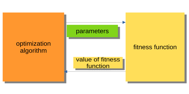
Fig. 1. Interaction between PSO and fitness function

The structure displayed in Fig. 2 is much more convenient. The optimization algorithm here is not an independent program, but a separate module or "black box". This module has 'min', 'max' and 'step' parameters for each optimized argument. The MQL program receives optimized arguments upon request and returns the fitness values or, in other words, the fitness function values. This structure allows building a range of very flexible solutions, from using automatic optimization in Expert Advisors to writing a custom optimization manager.

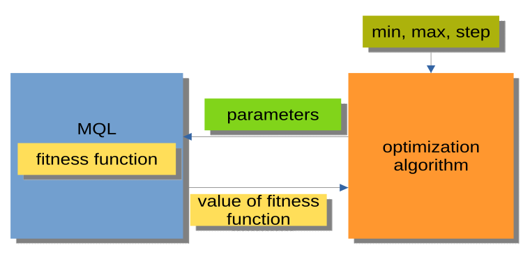
Fig 2. Interaction between MQL program and PSO

It is also worth mentioning that the organization of calls to methods of optimization algorithms (MQL block in Fig. 2) can be represented by a general scheme that is the same for all optimization algorithms (AO):

Thus, we see that only three public methods are used: Initialization_АО_0, Method_АО_1 and Method_АО_2. This is sufficient to organize the optimization process in user projects of any complexity.

The PSO workflow itself is shown in Figure 3 and includes the following logical steps:

1. Random particle generation (first iteration)
2. Obtaining the fitness value for each particle
3. Obtaining the fitness value for all particles in general
4. Particle speed adjustment
5. Breakpoint or going to step 2
   
6. Program completion.

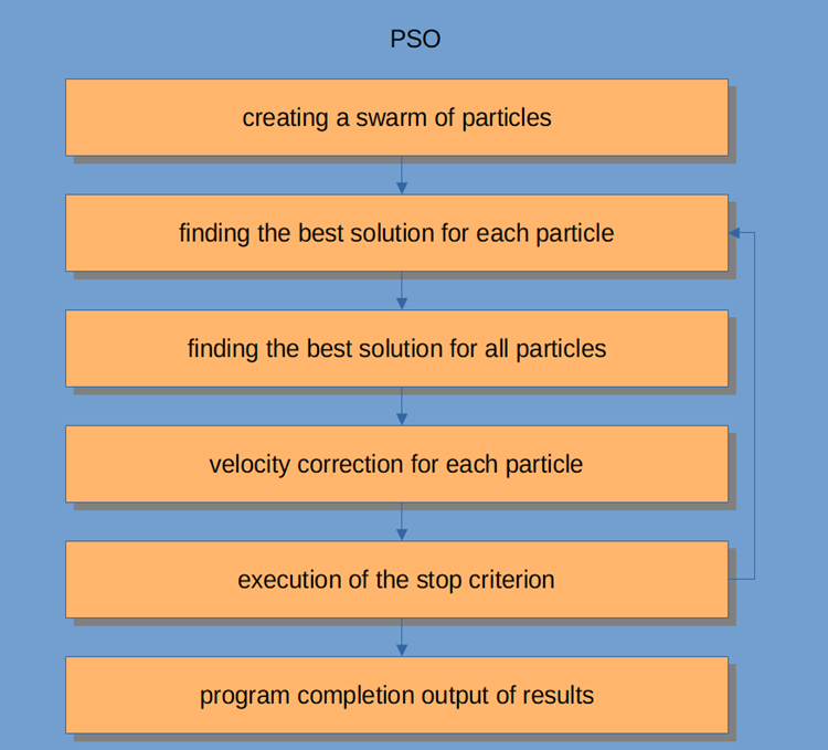
Fig. 3. PSO workflow

Let's consider the Particle Swarm algorithm in more detail.

The swarm intelligence system consists of many particles interacting both with each other and with the environment. Each particle follows simple rules, although there is no centralized behavior control system to tell each of them what to do. Local and random interactions between them lead to the emergence of intelligent group behavior that is not controlled by individuals.
If we draw an analogy with a flock, then we can say that all particles must perform simple tasks:

• avoid intersection with other particles;
• adjust their speed according to the speeds of the surrounding particles;
• try to keep a fairly small distance between themselves and the environment.

The PSO algorithm starts with a population initialization. The second step is to calculate the fitness values of each particle, after which the individual and global best scores are updated, and then the speed and position of the particles are updated. When using PSO, a possible solution to a numerical optimization problem is represented by the position of the particle. In addition, each particle has a current velocity that reflects its absolute magnitude and direction to a new, supposedly better, solution/position.

The particle also stores its fitness value, current position, best known position (a previous position with the best known fitness) and the fitness of the best known position. Steps two through four are repeated until the completion condition is met. In the first iteration, all particles are dispersed to find the best solution (exploration). Every particle is assessed. The best solutions for the neighborhood topology are found, and the personal and global best particles for each member of the swarm are updated. Convergence is achieved by attracting all particles to the particle with the best solution. 

Although the PSO algorithm is quite simple at its core, we need to understand it in order to be able to modify the code in this article to suit our needs. PSO is an iterative process. At each iteration in the main processing loop, the current speed of each particle is first updated. The current velocity of the particle, its local information and the global information of the swarm are taken into account. The position of each particle is then updated using the value of that particle's new velocity.

Mathematically, these two particle coordinate update equations look like this:

v(t+1) = w * v(t) + c1 * rp * (p(t) –  x(t)) + (c2 * rg * (g(t) –  x(t))

x(t+1) = x(t) + v(t+1)

The position update process is actually much simpler than the suggested equations. The first equation is for updating the particle's velocity.

The term v(t+1) denotes the speed at time t+1. The new speed depends on three terms.

• The first one: w * v(t). The w factor is called the weight fraction of inertia and is simply a constant; v(t) is the current speed at time t.
  
  
• The second term: c1 * rp * (p(t) – x(t)). The c1 factor is a constant called the cognitive (or personal, or local) weight fraction. The rp multiplier is a random variable in the [0, 1] range. The p(t) vector quantity is the particle's best position found so far, and the x(t) vector quantity is the particle's current position.
  
  
• The third term: speed update c2 * rg * (g(t) – x(t). The c2 factor is a constant called the social (or global) weight fraction. The rg multiplier is a random variable in the [0, 1] range. The value of the g(t) vector is the best known position found so far of any of the particles in the swarm. Once a new velocity is determined, v(t+1), it is used to calculate the particle's new position x(t+1).

3. Classic implementation

A logical unit describing a set of coordinates in space (optimized parameters) is a particle, which can be represented as a structure, where c[] are the coordinates of the particle, cB[] are the best coordinates of the particle for all iterations, v[] is the speed for each of coordinates of the particle, ff - the current fitness value of the particle, ffB - the best fitness value of the particle for all iterations. In the constructor of the particle structure, we initialize the values of ff and ffB using the minimum possible value that can be represented by the 'double' type, since the algorithm is designed to find the maximum of the function (to find the minimum, it is enough to add a "-" sign before the resulting fitness value).

//——————————————————————————————————————————————————————————————————————————————
struct S_Particles
{
  public:
    double c  []; //coordinates
    double cB []; //best coordinates
    double v  []; //velocity

    double ff;    //the value of the fitness function
    double ffB;   //best value fitness function

    S_Particles ()
    {
      ff  = -DBL_MAX;
      ffB = -DBL_MAX;
    }
};
//——————————————————————————————————————————————————————————————————————————————

Let's implement the PSO algorithm as a class featuring only three public methods InitPS (), Preparation () and Dwelling () (Initialization_АО_0, Method_АО_1 and Method_АО_2). Out of the private methods, GenerateRNDparticles () and ParticleMovement () are unique for PSO, while the rest have already been considered in the previous article. p [] structure array is a swarm of particles. In addition to the fact that each particle has fitness values, its own coordinates, and the best coordinates, the swarm as a whole has the best coordinates cB and the best fitness value ffB.

//——————————————————————————————————————————————————————————————————————————————
class C_AO_PSO
{
  public:
  //----------------------------------------------------------------------------
  S_Particles p    []; //particles
  double rangeMax  []; //maximum search range
  double rangeMin  []; //manimum search range
  double rangeStep []; //step search
  double cB        []; //best coordinates
  double ffB;          //FF of the best coordinates

  void InitPS (const int    params,       //number of opt. parameters
               const int    size,         //swarm size
               const double inertiaP,     //inertia
               const double selfBoostP,   //boost
               const double groupBoostP); //group boost

  void Preparation ();
  void Dwelling ();

  private:
  //----------------------------------------------------------------------------
  int swarmSize; //swarm size
  int parameters;//number of optimized parameters

  double inertia;
  double selfBoost;
  double groupBoost;
  bool   dwelling;

  void   GenerateRNDparticles ();
  void   ParticleMovement     ();
  double SeInDiSp             (double in, double inMin, double inMax, double step);
  double RNDfromCI            (double min, double max);
};
//——————————————————————————————————————————————————————————————————————————————

The InitPS () method is meant for initializing the algorithm before optimization starts (Initialization_АО_0). The method argument values are assigned to the private members in the method, as well as the size is assigned to the swarm and internal parameters of each particle in the swarm.

//——————————————————————————————————————————————————————————————————————————————
void C_AO_PSO::InitPS (const int    paramsP,
                       const int    sizeP,
                       const double inertiaP,
                       const double selfBoostP,
                       const double groupBoostP)
{
  ffB = -DBL_MAX;

  parameters = paramsP;
  swarmSize  = sizeP;

  ArrayResize (rangeMax,  parameters);
  ArrayResize (rangeMin,  parameters);
  ArrayResize (rangeStep, parameters);

  dwelling = false;

  inertia    = inertiaP;
  selfBoost  = selfBoostP;
  groupBoost = groupBoostP;

  ArrayResize (p, swarmSize);

  for (int i = 0; i < swarmSize; i++)
  {
    ArrayResize (p [i].c,  parameters);
    ArrayResize (p [i].cB, parameters);
    ArrayResize (p [i].v,  parameters);
  }

  ArrayResize (cB, parameters);
}
//——————————————————————————————————————————————————————————————————————————————

The Preparation () method is called at each iteration (epoch) first (Method_АО_1). The method is simple but very important. Depending on whether the method will be called on the first epoch or on subsequent epochs (determined by the dwelling flag), the swarm fitness value will be reset and a random swarm population will be created, or the particles will move to new coordinates.

//——————————————————————————————————————————————————————————————————————————————
void C_AO_PSO::Preparation ()
{
  if (!dwelling)
  {
    ffB = -DBL_MAX;
    GenerateRNDparticles ();
    dwelling = true;
  }
  else ParticleMovement ();
}
//——————————————————————————————————————————————————————————————————————————————

A random swarm population is generated in the GenerateRNDparticles () method. The particles have random coordinates in the range specified for each of them, and a random speed for each of the coordinates.

//——————————————————————————————————————————————————————————————————————————————
void C_AO_PSO::GenerateRNDparticles ()
{
  for (int s = 0; s < swarmSize; s++)
  {
    for (int k = 0; k < parameters; k++)
    {
      p [s].c  [k] = RNDfromCI (rangeMin [k], rangeMax [k]);
      p [s].c  [k] = SeInDiSp (p [s].c [k], rangeMin [k], rangeMax [k], rangeStep [k]);
      p [s].cB [k] = p [s].c [k];
      p [s].v  [k] = RNDfromCI (0.0, (rangeMax [k] - rangeMin [k]) * 0.5);
    }
  }
}
//——————————————————————————————————————————————————————————————————————————————

The ParticleMovement () method triggers the algorithm for moving particles to new positions. To achieve this, it is necessary to calculate the speed for each coordinate according to the above equation. I do not know why the term "velocity" is used, as it is basically a displacement value, or in other words, the difference between where the particle is at the moment and where it should be moving. Having calculated this difference for each of the coordinates, we simply add to the current values. After that, check if it unacceptable to go beyond the min/max boundaries of the optimized parameters (for a particle, these are coordinates) with a given step.

//——————————————————————————————————————————————————————————————————————————————
void C_AO_PSO::ParticleMovement ()
{
  double rp;       //random component of particle movement
  double rg;
  double velocity;
  double posit;
  double positBest;
  double groupBest;

  for (int i = 0; i < swarmSize; i++)
  {
    for (int k = 0; k < parameters; k++)
    {
      rp = RNDfromCI (0.0, 1.0);
      rg = RNDfromCI (0.0, 1.0);
      
      velocity  = p [i].v  [k];
      posit     = p [i].c  [k];
      positBest = p [i].cB [k];
      groupBest = cB [k];

      p [i].v [k] = inertia * velocity + selfBoost * rp * (positBest - posit) + groupBoost * rg * (groupBest - posit);
      p [i].c [k] = posit + p [i].v [k];

      p [i].c [k] = SeInDiSp (p [i].c [k], rangeMin [k], rangeMax [k], rangeStep [k]);
    }
  }
}
//——————————————————————————————————————————————————————————————————————————————

The Dwelling () method is the third public method of the algorithm used for optimization (Method_АО_2). The purpose of the method is to update the best coordinates and fitness values of each particle relative to its previous performance, as well as update the fitness of the swarm and the best coordinates of the swarm if necessary. The method is called after getting the fitness values in the iteration loop.

//——————————————————————————————————————————————————————————————————————————————
void C_AO_PSO::Dwelling ()
{
  for (int i = 0; i < swarmSize; i++)
  {
    //remember the best position for the particle
    if (p [i].ff > p [i].ffB)
    {
      p [i].ffB = p [i].ff;
      for (int k = 0; k < parameters; k++) p [i].cB [k] = p [i].c [k];
    }

    if (p [i].ff > ffB)
    {
      ffB = p [i].ff;
      for (int k = 0; k < parameters; k++) cB [k] = p [i].c [k];
    }
  }
}
//——————————————————————————————————————————————————————————————————————————————

The function for discretization of the 'double' number with a given step in the specified range.

//——————————————————————————————————————————————————————————————————————————————
// Choice in discrete space
double C_AO_PSO::SeInDiSp (double in, double inMin, double inMax, double step)
{
  if (in <= inMin) return (inMin);
  if (in >= inMax) return (inMax);
  if (step == 0.0) return (in);
  else return (inMin + step * (double)MathRound ((in - inMin) / step));
}
//——————————————————————————————————————————————————————————————————————————————

The function for getting a random 'double' number in a specified range.

//——————————————————————————————————————————————————————————————————————————————
// Random number generator in the custom interval
double C_AO_PSO::RNDfromCI (double min, double max)
{
  if (min == max) return (min);
  double Min, Max;
  if (min > max)
  {
    Min = max;
    Max = min;
  }
  else
  {
    Min = min;
    Max = max;
  }
  return (double(Min + ((Max - Min) * (double)MathRand () / 32767.0)));
}
//——————————————————————————————————————————————————————————————————————————————

The theory is over. Let's get down to practice.

Since I use the same structure for constructing algorithms as in the first article of the series (and I will continue doing this in the future) described in Fig. 2, then it will not be difficult for us to connect the algorithm to the test stand.

When running the stand, we will see animations similar to those shown below. In this case, we can clearly see how a swarm of particles behaves. The swarm behaves really like a swarm in nature. On the heat map of the function, it moves in the form of a dense cloud.

As you might remember, the black circle denotes the global optimum (max) of the function, while the black dot denotes the best average coordinates of the search algorithm obtained at the time of the current iteration. Let me explain where the average values come from. The heat map is two-dimensional in coordinates, and the function being optimized can include hundreds of variables (measurements). Therefore, the result is averaged by coordinates.

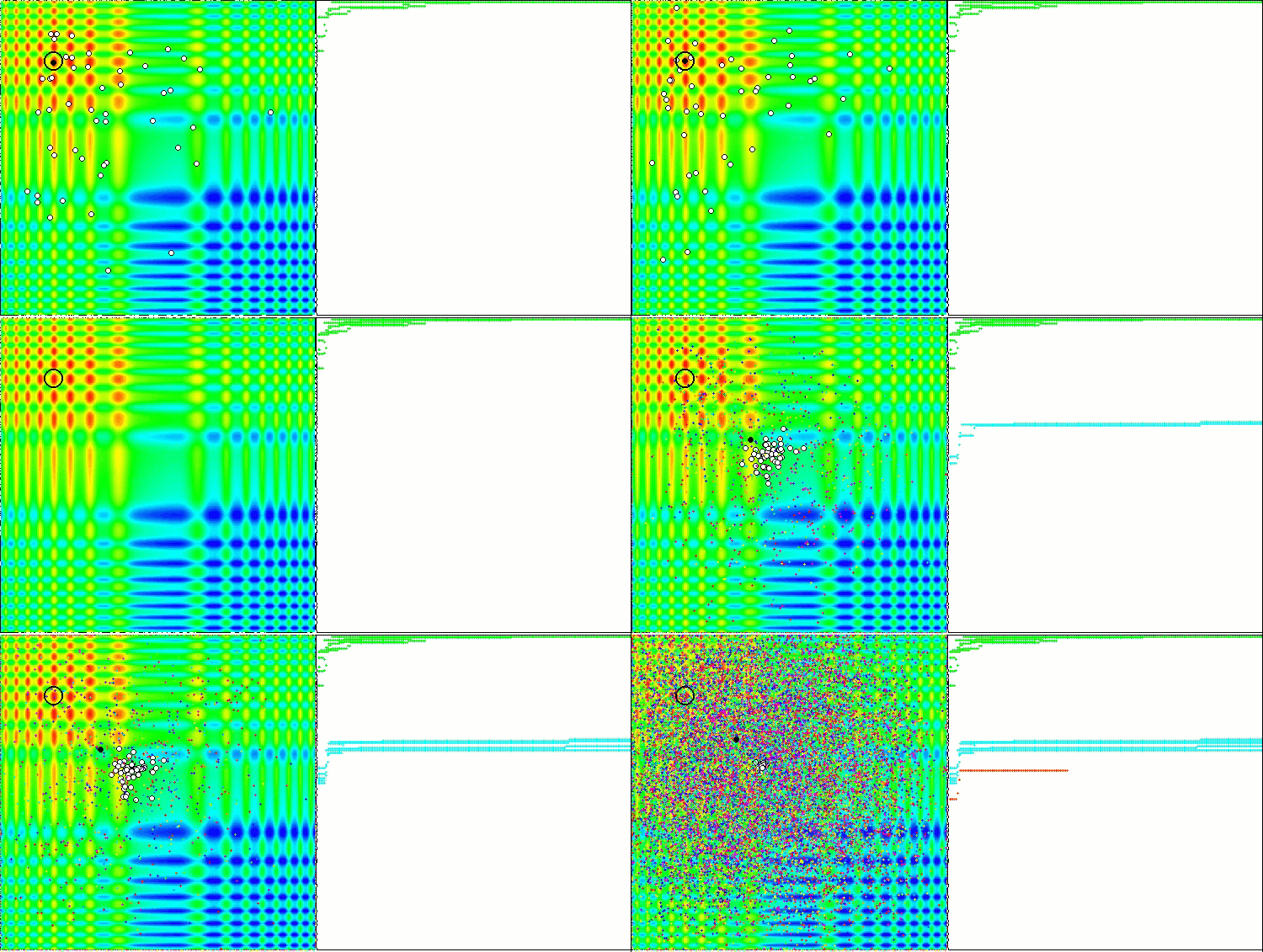
  PSO on the Skin test function.

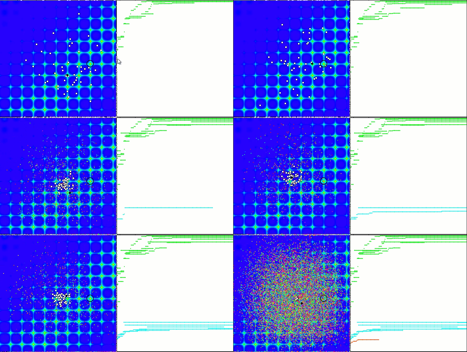
  PSO on the Forest test function.

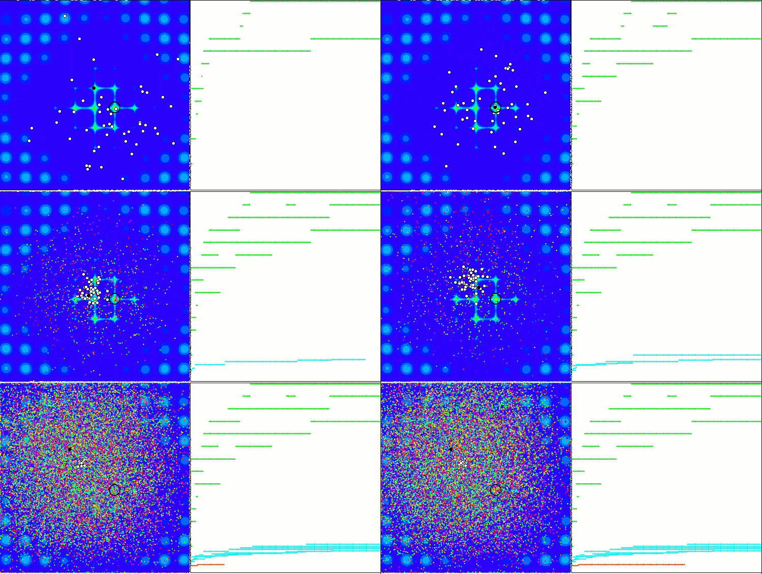
  PSO on the Megacity test function.

As you can see in the animation, the tests showed that PSO copes quite well with the smooth first function, but only when optimizing two variables. With an increase in the dimension of the search space, the efficiency of the algorithm drops sharply. This is especially noticeable on the second and discrete third functions. The results are noticeably worse than the random algorithm described in the previous article. We will return to the results and discuss them in detail when forming a comparative table of results.

Looking at how the famous PSO algorithm shamefully loses to random one, one might want to give the algorithm a second chance. In the next section, I will try to modify the PSO algorithm.

4. Modified version

In my opinion, the weaknesses of PSO are:

1) Each of the coordinates will necessarily be changed with the probability of almost equal to 1. This means that each particle of the swarm, at each iteration, oscillates, at best, somewhere in the local extremum of the global region, while at worst, it never hits exactly the point of the global extremum. This implies a characteristic feature of the algorithm - getting stuck in local extrema, i.e. bad convergence.

2) The algorithm does not work well with discrete functions, partly because of the first flaw. Particle coordinates jump to the nearest "areas" of the surface of the function being optimized, not being able to study in detail the neighborhood of any local extremum.

3) Weak ability of the algorithm to explore new areas. The swarm focuses somewhere in one place without trying to escape the local "hole". Some authors mention attempts to create an implementation of a multi-swarm modification, but the questions of optimizing complex multi-variable functions remain open, since the principle of mutual distance is unclear, because not only the principle of joint movement must be fulfilled, but also the possibility of mutual repulsion. Otherwise, there is no point in such an implementation because individual swarms will simply converge in one area or point. At the same time, the optimization of simple one- or two-variable functions is performed by the simplest methods with excellent convergence.

So what can we do to improve the algorithm?

It is obvious (although not necessarily true) that we need to pass the best individual coordinates to particles from other particles. The better the overall coordinates of the "donor" particle, the greater the probability of passing the coordinates. The shift in the probability of choosing a particle is schematically shown in Fig. 4. We generate a random number from 0 to 1, transform the resulting number with a parabolic function, and then scale it to the range of serial numbers of particles in the swarm from 0 to SwarmSize-1. To do this, we need to introduce an additional parameter for PSOm (the modified algorithm) - the probability of copying the coordinate, and we also need to sort the swarm so that the better the particle, the closer it is to index 0.

Fig. 4. Shifted particle selection probability

Let's slightly change the ParticleMovement () method. Generate a random number [0;1]. if the number turns out to be greater than the 'copy' parameter, then we will perform the usual operations with the particle described in detail above, otherwise we will copy the coordinate of another particle with the index chosen according to the rule graphically shown in Fig. 4.

//——————————————————————————————————————————————————————————————————————————————
void C_AO_PSOm::ParticleMovement ()
{
  double rp;       //random component of particle movement
  double rg;
  double velocity;
  double posit;
  double positBest;
  double groupBest;

  for (int i = 0; i < swarmSize; i++)
  {
    for (int k = 0; k < parameters; k++)
    {
      rp = RNDfromCI (0.0, 1.0);
      rg = RNDfromCI (0.0, 1.0);

      double rC = RNDfromCI (0.0, 1.0);

      if (rC > copy)
      {
        velocity  = p [i].v  [k];
        posit     = p [i].c  [k];
        positBest = p [i].cB [k];
        groupBest = cB [k];

        p [i].v [k] = inertia * velocity + selfBoost * rp * (positBest - posit) + groupBoost * rg * (groupBest - posit);
        p [i].c [k] = posit + p [i].v [k];

        p [i].c [k] = SeInDiSp (p [i].c [k], rangeMin [k], rangeMax [k], rangeStep [k]);
      }
      else p [i].c [k] = p [GetPartcileAdress ()].cB [k];
    }
  }
}
//——————————————————————————————————————————————————————————————————————————————

The Dwelling () method should be changed as well. Add calling the SortParticles () sorting function.

//——————————————————————————————————————————————————————————————————————————————
void C_AO_PSOm::Dwelling ()
{
  for (int i = 0; i < swarmSize; i++)
  {
    //remember the best position for the particle
    if (p [i].ff > p [i].ffB)
    {
      p [i].ffB = p [i].ff;
      for (int k = 0; k < parameters; k++) p [i].cB [k] = p [i].c [k];
    }

    if (p [i].ff > ffB)
    {
      ffB = p [i].ff;
      for (int k = 0; k < parameters; k++) cB [k] = p [i].c [k];
    }
  }

  SortParticles ();
}
//——————————————————————————————————————————————————————————————————————————————

The GetParticleAdress () function provides a choice of the address of a particle with a probability shifted towards the best particle.

//——————————————————————————————————————————————————————————————————————————————
//shift of probability in the smaller party (to an index 0)
int C_AO_PSOm::GetParticleAdress ()
{
  double x = RNDfromCI (-1.0, 0.0);
  x = x * x;
  x = Scale (x, 0.0, 1.0, 0, swarmSize - 1);
  x = SeInDiSp (x, 0, swarmSize - 1, 1);
  return ((int)x);
}
//——————————————————————————————————————————————————————————————————————————————

The SortParticles () function is a conventional bubble sorting.

//——————————————————————————————————————————————————————————————————————————————
//Sorting of particles
void C_AO_PSOm::SortParticles ()
{
  //----------------------------------------------------------------------------
  int   cnt = 1;
  int   t0 = 0;
  double t1 = 0.0;
  //----------------------------------------------------------------------------

  // We will put indexes in the temporary array
  for (int i = 0; i < swarmSize; i++)
  {
    ind [i] = i;
    val [i] = p [i].ffB; //ffPop [i];
  }

  while (cnt > 0)
  {

    cnt = 0;
    for (int i = 0; i < swarmSize - 1; i++)
    {
      if (val [i] < val [i + 1])
      {
        t0 = ind [i + 1];
        t1 = val [i + 1];
        ind [i + 1] = ind [i];
        val [i + 1] = val [i];
        ind [i] = t0;
        val [i] = t1;

        cnt++;
      }
    }
  }

  // On the received indexes create the sorted temporary population
  for (int u = 0; u < swarmSize; u++) pT [u] = p [ind [u]];

  // Copy the sorted array back
  for (int u = 0; u < swarmSize; u++) p [u] = pT [u];
}
//——————————————————————————————————————————————————————————————————————————————

The function for scaling a number from one numerical range to another.

//——————————————————————————————————————————————————————————————————————————————
double C_AO_PSOm::Scale (double In, double InMIN, double InMAX, double OutMIN, double OutMAX)
{
  if (OutMIN == OutMAX) return (OutMIN);
  if (InMIN == InMAX) return (double((OutMIN + OutMAX) / 2.0));
  else
  {
    if (In < InMIN) return (OutMIN);
    if (In > InMAX) return (OutMAX);
    return (((In - InMIN) * (OutMAX - OutMIN) / (InMAX - InMIN)) + OutMIN);
  }
}
//——————————————————————————————————————————————————————————————————————————————

5. Test results

Finally, let's summarize the results of the current research. Unfortunately, the PSO algorithm did not justify itself no matter how much I would like to hope for good results. The studies showed its weak convergence for discrete functions with breaks and with a large number of arguments. An attempt to modify the algorithm was unsuccessful, the results turned out to be even worse than those of the classical implementation.

Increasing the copy parameter to values close to 0.8 is still able to show instant convergence but only for the first smooth function in the tests and with only two arguments. For other tests, this parameter only worsens the results. The classic implementation of PSO managed to show something interesting only on the Skin function with 1000 arguments. Other tests turned out to be mediocre.

The final test result is 0.47695 for the classic algorithm and 0.45144 for the modified one respectively. The results are shown in the table below. The test stand allows us to select the number of test runs in the settings (default is 5), so readers can get statistically more accurate results by setting this parameter higher if allowed by computing power.

AO	Runs	Skin			Forest			Megacity (discrete)			Final result
		2 params (1 F)	40 params (20 F)	1000 params (500 F)	2 params (1 F)	40 params (20 F)	1000 params (500 F)	2 params (1 F)	40 params (20 F)	1000 params (500 F)
RND	1000	0.98744	0.61852	0.49408	0.89582	0.19645	0.14042	0.77333	0.19000	0.14283	0.51254
	10,000	0.99977	0.69448	0.50188	0.98181	0.24433	0.14042	0.88000	0.20133	0.14283
PSO	1000	0.98436	0.72243	0.65483	0.71122	0.15603	0.08727	0.53333	0.08000	0.04085	0.47695
	10,000	0.99836	0.72329	0.65483	0.97615	0.19640	0.09219	0.82667	0.10600	0.04085
PSOm	1000	0.96678	0.64727	0.57654	0.80616	0.13388	0.06800	0.53333	0.08067	0.04211	0.45144
	10,000	0.99505	0.64986	0.57654	0.90401	0.18194	0.07104	0.74667	0.10400	0.04211

Summarizing all of the above, PSO tends to lead to fast and premature convergence at average optimal points in addition to slow convergence in the refined search area (having poor local search ability). Simply put, the algorithm is very weak and is not suitable for optimizing complex and even more so discrete functions, especially functions of multiple arguments.

There are several approaches that can be used to improve PSO in general. Swarm size is one of the important factors. A higher swarm size can increase the likelihood of faster and more accurate convergence. However, in practical problems there is often a threshold on the number of runs of the fitness function, and increasing the swarm size will only proportionally reduce the number of epochs, and therefore reduce the possibility of swarm evolution.

The second approach is to strike a balance between exploration and exploitation. At the beginning of the iterations, the high degree of exploration would give a high chance of finding a solution close to the global optimum. Meanwhile, by the end of the iteration, a high degree of exploitation would give the particle a chance to find the most accurate solution in the promising area. Pre-optimization before the swarm stage by other methods is another technique that can be used to improve the underlying performance of PSO, which is quite commonly used nowadays. Assigning different tasks or goals to each subgroup can also increase the effectiveness of the PSO in multi-task problems. 

Another approach to improve the performance of the PSO is to establish the constituent components of the velocity equation (dynamic speed control). Such an approach can send particles in different directions and lead to faster convergence to the global optimum, but this is just an assumption.