Data Science and Machine Learning (Part 06): Gradient Descent
Omega J Msigwa | 27 July, 2022
Premature optimization is the root of all evil in programming
-Donald Knuth
Introduction
According to Wikipedia gradient descent (also often called steepest descent) is a first-order iterative optimization algorithm for finding a local minimum of a differentiable function. The idea is to take repeated steps in the opposite direction of the gradient (or approximate gradient) of the function at the current point, because this is the direction of steepest descent. Conversely, stepping in the direction of the gradient will lead to a local maximum of that function; the procedure is then known as gradient ascent. Basically, the gradient descent is an optimization algorithm used to find the minimum of a function:

The gradient descent is a very important algorithm in machine learning as it helps us find the parameters for the best model for our dataset. Let me first explain the term Cost Function.
Cost Function
Some folks call this loss function, it is a metric for calculating how good or bad our model is at predicting the relationship between the values of x and y.
There are a lot of metrics that can be used to determine how the model is predicting but unlike all those, the cost function finds the average loss over the entire dataset, the larger the cost function the bad our model is at finding the relationships in our dataset.
Gradient Descent aims at minimizing the cost function because the model with the lowest cost function is the best model. For you to understand what I just explained let's see this following example.
Suppose our cost function is the equation
![]()
If we plot a graph of this function with python this is how it will look like this:

The very first step we need to do to our cost function is to differentiate the cost function, using the Chain Rule:
The equation y= (x+5)^2 is a composite function (there is one function inside of another). The outer function being (x+5)^2 the Inner function being (x+5). To differentiate this let's apply the Chain rule, see the image:

There is a video linked at the end of me doing the maths by hand, if you found this hard to understand. Ok so now this function that we just obtained is the Gradient. The process of finding the gradient of an equation is the most important step of all of them and I wish my mathematical teachers told me back in the day that the purpose of differentiating the function is so that we get the gradient of a function.
That is the first and most important step, below is the second step.
Step 02:
We move in the negative direction of the gradient, here the question raises, how much should we move? This is where the learning rate comes into play.
Learning Rate
By definition, this is the step size at each iteration while moving toward a minimum of a loss function, take an example of a person stepping down the mountain, their steps are the learning rate, the smaller the steps the longer it will take them to reach the bottom of the mountain and vice versa.
Keep the algorithm learning rate to smaller values but not very small like 0.0001 by doing so you are increasing the program execution time as it might take longer for the algorithm to reach the minimum values. In contrast, using big numbers for the learning rate will cause the algorithm to skip the minimum values which in the end may cause you to miss the minimum value targeted.
The default learning rate is 0.01.
Let's perform the iteration to see how the algorithm works.
First Iteration: We choose any random point as a starting point for our algorithm, I chose 0 as a the first value of x now, to update the values of x this is the formula

By each iteration, we will descend toward the minimum value of the function and so is the name Gradient Descent. Making sense now?

Let's see how this works in details. Now let's calculate the values manually on 2 iterations so that you get a solid understanding on what's happening:
1st Iteration:
formula: x1 = x0 - learning rate * ( 2*(x+5) )
x1 = 0 - 0.01 * 0.01 * 2*(0+5)
x1 = -0.01 * 10
x1 = -0.1 (finally)
Now the finally we update the values by assigning the new value to the old value and repeat the procedure for as much iterations until we reach the minimum of a function:
x0 = x1
2nd Iteration:
x1 = -0.1 - 0.01 * 2*(-0.1+5)
x1 = -0.198
Then: x0 = x1
If we repeat this procedure a several times the output for 10 first iterations will be:
RS      0       17:15:16.793    gradient-descent test (EURUSD,M1)       Gradient Descent CostFunction CUSTOM
QQ      0       17:15:16.793    gradient-descent test (EURUSD,M1)       1 x0 = 0.0000000000 x1 = -0.1000000000 CostFunction = 10.0000000000
ES      0       17:15:16.793    gradient-descent test (EURUSD,M1)       2 x0 = -0.1000000000 x1 = -0.1980000000 CostFunction = 9.8000000000
PR      0       17:15:16.793    gradient-descent test (EURUSD,M1)       3 x0 = -0.1980000000 x1 = -0.2940400000 CostFunction = 9.6040000000
LE      0       17:15:16.793    gradient-descent test (EURUSD,M1)       4 x0 = -0.2940400000 x1 = -0.3881592000 CostFunction = 9.4119200000
JD      0       17:15:16.793    gradient-descent test (EURUSD,M1)       5 x0 = -0.3881592000 x1 = -0.4803960160 CostFunction = 9.2236816000
IG      0       17:15:16.793    gradient-descent test (EURUSD,M1)       6 x0 = -0.4803960160 x1 = -0.5707880957 CostFunction = 9.0392079680
IG      0       17:15:16.793    gradient-descent test (EURUSD,M1)       7 x0 = -0.5707880957 x1 = -0.6593723338 CostFunction = 8.8584238086
JF      0       17:15:16.793    gradient-descent test (EURUSD,M1)       8 x0 = -0.6593723338 x1 = -0.7461848871 CostFunction = 8.6812553325
NI      0       17:15:16.793    gradient-descent test (EURUSD,M1)       9 x0 = -0.7461848871 x1 = -0.8312611893 CostFunction = 8.5076302258
CK      0       17:15:16.793    gradient-descent test (EURUSD,M1)       10 x0 = -0.8312611893 x1 = -0.9146359656 CostFunction = 8.3374776213
Let's also see the other ten values of the algorithm when it is very close to the minimum of the function:
GK      0       17:15:16.800    gradient-descent test (EURUSD,M1)       1052 x0 = -4.9999999970 x1 = -4.9999999971 CostFunction = 0.0000000060
IH      0       17:15:16.800    gradient-descent test (EURUSD,M1)       1053 x0 = -4.9999999971 x1 = -4.9999999971 CostFunction = 0.0000000059
NH      0       17:15:16.800    gradient-descent test (EURUSD,M1)       1054 x0 = -4.9999999971 x1 = -4.9999999972 CostFunction = 0.0000000058
QI      0       17:15:16.800    gradient-descent test (EURUSD,M1)       1055 x0 = -4.9999999972 x1 = -4.9999999972 CostFunction = 0.0000000057
II      0       17:15:16.800    gradient-descent test (EURUSD,M1)       1056 x0 = -4.9999999972 x1 = -4.9999999973 CostFunction = 0.0000000055
RN      0       17:15:16.800    gradient-descent test (EURUSD,M1)       1057 x0 = -4.9999999973 x1 = -4.9999999973 CostFunction = 0.0000000054
KN      0       17:15:16.800    gradient-descent test (EURUSD,M1)       1058 x0 = -4.9999999973 x1 = -4.9999999974 CostFunction = 0.0000000053
JO      0       17:15:16.800    gradient-descent test (EURUSD,M1)       1059 x0 = -4.9999999974 x1 = -4.9999999974 CostFunction = 0.0000000052
JO      0       17:15:16.800    gradient-descent test (EURUSD,M1)       1060 x0 = -4.9999999974 x1 = -4.9999999975 CostFunction = 0.0000000051
QL      0       17:15:16.800    gradient-descent test (EURUSD,M1)       1061 x0 = -4.9999999975 x1 = -4.9999999975 CostFunction = 0.0000000050
QL      0       17:15:16.800    gradient-descent test (EURUSD,M1)       1062 x0 = -4.9999999975 x1 = -4.9999999976 CostFunction = 0.0000000049
HP      0       17:15:16.800    gradient-descent test (EURUSD,M1)       Local miminum found =-4.999999997546217
After 1062 (One thousand and sixty two) iterations the algorithm was able to reach the local minimum of this function.
A thing to notice from this algorithm
Looking at the values of Cost Function you will notice huge change in values at the beginning, but very tiny noticeable changes to the last values of a cost function.
The gradient descent takes larger steps when it is nowhere near the minimum of a function but, takes baby steps when is is near the minimum of the function, the same thing you will do when you are near the bottom of the mountain, so now you know that the gradient descent is pretty smart!
In the end the local minimum is
HP 0 17:15:16.800 gradient-descent test (EURUSD,M1) Local miminum found =-4.999999997546217
Which is the accurate value because the minimum of this function is -5.0!
The Real Question
How does the Gradient know when to stop? See we can let the algorithm keep on iterating till infinity or at least the end of a computer's ability to calculate.
When the cost function is Zero is when we know that the gradient descent has done it's job.
Now let's code this whole operation in MQL5:
       while (true)
        {
           iterations++;

           x1 = x0 - m_learning_rate * CustomCostFunction(x0);

           printf("%d x0 = %.10f x1 = %.10f CostFunction = %.10f",iterations,x0,x1,CustomCostFunction(x0));

           if (NormalizeDouble(CustomCostFunction(x0),8) == 0) { Print("Local minimum found =",x0);  break;  }

           x0 = x1;
        }
The above block of code is the one that was able to get us the results we wanted but it's not alone in the class CGradientDescent. The Function CustomCostFunction is where our differentiated equation was being kept and calculated here it is
double CGradientDescent::CustomCostFunction(double x)
 {
   return(2 * ( x + 5 ));
 }
What's the Purpose?
One might be asking themselves what's the purpose of all these calculations when you can just use the default linear model created by the previous libraries we discussed in this article series. Newsflash the model created using the default values isn't necessarily the best model so you need to let the computer learn the best parameters for the model with few errors (best model).
We are a few articles closer to building Artificial Neural Networks and for everyone to be able to understand how neural networks learn (teach themselves the patterns) in the process of back propagations and other techniques, gradient descent is the most popular algorithm that has made all that possible. Without a solid understanding of it you may never understand the process because things are about to get complicated.
Gradient Descent for a Regression Model
Using the Salary Dataset let's build get the best model using the gradient descent.

Data visualization in Python:
import pandas as pd
import numpy as np
import matplotlib.pyplot as plt


data  = pd.read_csv(r"C:\Users\Omega Joctan\AppData\Roaming\MetaQuotes\Terminal\892B47EBC091D6EF95E3961284A76097\MQL5\Files\Salary_Data.csv")

print(data.head(10))

x = data["YearsExperience"]
y = data["Salary"]

plt.figure(figsize=(16,9))
plt.title("Experience vs Salary")
plt.scatter(x,y,c="green")
plt.xlabel(xlabel="Years of Experience")
plt.ylabel(ylabel="Salary")
plt.show()
This will be our graph:

Looking at our dataset you can not help but notice that this dataset is for a regression problem, but we can have a million number of models to help us make the prediction or whatever it is we are trying to achieve.

What is the Best model to use to make predictions of a person's experience and what their salary will be, that's what we are going to find out. But first let's derive the cost function for our regression model.
Theory
Let me take you back to Linear Regression.
We know for a fact that every linear model has errors associated with it. We also know that we can create a million lines in this graph and the best fit line is always the line with the least errors.
The cost function represents the error between our actual values and predicted values, we can write the formula for the cost function to be equal to:
Cost = Y Actual - Y Predicted
Since we are seeing the magnitude of errors we raise the square, our formula now becomes
![]()
But we are looking for Errors in our entire Dataset, we need to make the summation
![]()
Finally, we divide the summation of errors by the m which is the number of items in the dataset :

Here is the video on the whole mathematical procedures done by hand.
Now that we have the cost function let's code for the gradient descent and find the best parameters for both. Coefficient of X(Slope) denoted as Bo and The Y Intercept denoted as B1
   double cost_B0=0, cost_B1=0;

   if (costFunction == MSE)
    {
      int iterations=0;
      for (int i=0; i<m_iterations; i++, iterations++)
        {

           cost_B0 = Mse(b0,b1,Intercept);
           cost_B1 = Mse(b0,b1,Slope);

           b0 = b0 - m_learning_rate * cost_B0;
           b1 = b1 - m_learning_rate * cost_B1;

           printf("%d b0 = %.8f cost_B0 = %.8f B1 = %.8f cost_B1 = %.8f",iterations,b0,cost_B0,b1,cost_B1);

           DBL_MAX_MIN(b0); DBL_MAX_MIN(cost_B0); DBL_MAX_MIN(cost_B1);

           if (NormalizeDouble(cost_B0,8) == 0 && NormalizeDouble(cost_B1,8) == 0)  break;

        }
      printf("%d Iterations Local Minima are\nB0(Intercept) = %.5f  ||  B1(Coefficient) = %.5f",iterations,b0,b1);
    }
Notice a few things from the Gradient Descent code:
- The process is still the same as the one we performed before but this time we are finding and updating the values twice at once the Bo and B1.
- There is a restricted number of iterations, someone once said the best way to make an infinite loop is to use a while loop we do not use the while loop this time but instead we want to limit the number of times the algorithm will work out to find the coefficients for the best model.
- DBL_MAX_MIN is a function for debugging purpose responsible to check and notify us if we have hit the mathematical limits of a computer.
This is the output of the operations of the algorithm. Learning Rate = 0.01 Iterations = 10000
PD      0       17:29:17.999    gradient-descent test (EURUSD,M1)       [20]  91738.0000  98273.0000 101302.0000 113812.0000 109431.0000 105582.0000 116969.0000 112635.0000 122391.0000 121872.0000
JS      0       17:29:17.999    gradient-descent test (EURUSD,M1)       Gradient Descent CostFunction MSE
RF      0       17:29:17.999    gradient-descent test (EURUSD,M1)       0 b0 = 1520.06000000 cost_B0 = -152006.00000000 B1 = 9547.97400000 cost_B1 = -954797.40000000
OP      0       17:29:17.999    gradient-descent test (EURUSD,M1)       1 b0 = 1995.08742960 cost_B0 = -47502.74296000 B1 = 12056.69235267 cost_B1 = -250871.83526667
LP      0       17:29:17.999    gradient-descent test (EURUSD,M1)       2 b0 = 2194.02117366 cost_B0 = -19893.37440646 B1 = 12707.81767044 cost_B1 = -65112.53177770
QN      0       17:29:17.999    gradient-descent test (EURUSD,M1)       3 b0 = 2319.78332575 cost_B0 = -12576.21520809 B1 = 12868.77569178 cost_B1 = -16095.80213357
LO      0       17:29:17.999    gradient-descent test (EURUSD,M1)       4 b0 = 2425.92576238 cost_B0 = -10614.24366387 B1 = 12900.42596039 cost_B1 = -3165.02686058
GH      0       17:29:17.999    gradient-descent test (EURUSD,M1)       5 b0 = 2526.58198175 cost_B0 = -10065.62193621 B1 = 12897.99808257 cost_B1 = 242.78778134
CJ      0       17:29:17.999    gradient-descent test (EURUSD,M1)       6 b0 = 2625.48307920 cost_B0 = -9890.10974571 B1 = 12886.62268517 cost_B1 = 1137.53974060
DD      0       17:29:17.999    gradient-descent test (EURUSD,M1)       7 b0 = 2723.61498028 cost_B0 = -9813.19010723 B1 = 12872.93147573 cost_B1 = 1369.12094310
HF      0       17:29:17.999    gradient-descent test (EURUSD,M1)       8 b0 = 2821.23916252 cost_B0 = -9762.41822398 B1 = 12858.67435081 cost_B1 = 1425.71249248

<<<<<<<<<<<<<<<<<<<<<<<<<<<<<<<<<<<<<<<< Last Iterations >>>>>>>>>>>>>>>>>>>>>>>>>>>>>>>>>>>>>>>>>>>>>>>>>>>>>>>>>>>>>>>>

EI      0       17:29:48.247    gradient-descent test (EURUSD,M1)       6672 b0 = 25792.20019866 cost_B0 = -0.00000001 B1 = 9449.96232146 cost_B1 = 0.00000000
NG      0       17:29:48.247    gradient-descent test (EURUSD,M1)       6673 b0 = 25792.20019866 cost_B0 = -0.00000001 B1 = 9449.96232146 cost_B1 = 0.00000000
GD      0       17:29:48.247    gradient-descent test (EURUSD,M1)       6674 b0 = 25792.20019866 cost_B0 = -0.00000001 B1 = 9449.96232146 cost_B1 = 0.00000000
PR      0       17:29:48.247    gradient-descent test (EURUSD,M1)       6675 b0 = 25792.20019866 cost_B0 = -0.00000001 B1 = 9449.96232146 cost_B1 = 0.00000000
IS      0       17:29:48.247    gradient-descent test (EURUSD,M1)       6676 b0 = 25792.20019866 cost_B0 = -0.00000001 B1 = 9449.96232146 cost_B1 = 0.00000000
RQ      0       17:29:48.247    gradient-descent test (EURUSD,M1)       6677 b0 = 25792.20019866 cost_B0 = -0.00000001 B1 = 9449.96232146 cost_B1 = 0.00000000
KN      0       17:29:48.247    gradient-descent test (EURUSD,M1)       6678 b0 = 25792.20019866 cost_B0 = -0.00000001 B1 = 9449.96232146 cost_B1 = 0.00000000
DL      0       17:29:48.247    gradient-descent test (EURUSD,M1)       6679 b0 = 25792.20019866 cost_B0 = -0.00000001 B1 = 9449.96232146 cost_B1 = 0.00000000
RM      0       17:29:48.247    gradient-descent test (EURUSD,M1)       6680 b0 = 25792.20019866 cost_B0 = -0.00000001 B1 = 9449.96232146 cost_B1 = 0.00000000
IK      0       17:29:48.247    gradient-descent test (EURUSD,M1)       6681 b0 = 25792.20019866 cost_B0 = -0.00000001 B1 = 9449.96232146 cost_B1 = 0.00000000
PH      0       17:29:48.247    gradient-descent test (EURUSD,M1)       6682 b0 = 25792.20019866 cost_B0 = -0.00000001 B1 = 9449.96232146 cost_B1 = 0.00000000
GF      0       17:29:48.247    gradient-descent test (EURUSD,M1)       6683 b0 = 25792.20019866 cost_B0 = -0.00000001 B1 = 9449.96232146 cost_B1 = 0.00000000
MG      0       17:29:48.247    gradient-descent test (EURUSD,M1)       6684 b0 = 25792.20019866 cost_B0 = -0.00000000 B1 = 9449.96232146 cost_B1 = 0.00000000
LE      0       17:29:48.247    gradient-descent test (EURUSD,M1)       6684 Iterations Local Minima are
OJ      0       17:29:48.247    gradient-descent test (EURUSD,M1)       B0(Intercept) = 25792.20020  ||  B1(Coefficient) = 9449.96232
If we plot the graph using matplotlib

B A M, The gradient Descent has been able to successfully get the best model out of 10000 models we tried out, great but there is one crucial step we are missing out that may cause our model to behave strangely and make us get the results we do not want.
Normalizing Linear Regression Input Variables Data
We know that for different datasets the best models can be found after different iterations some may take 100 iterations to reach the best models and some could take 10000 or up to a million iterations for the cost function to become zero not to mention that if we get the learning rate wrong values we may end up missing the local minima and if we miss that target we will end up hitting mathematical limits of a computer, let's see this in practice.
Learning Rate = 0.1 Iterations 1000
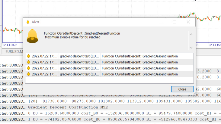
We just hit the maximum double value allowed by the system. Here are our logs.
GM      0       17:28:14.819    gradient-descent test (EURUSD,M1)       Gradient Descent CostFunction MSE
OP      0       17:28:14.819    gradient-descent test (EURUSD,M1)       0 b0 = 15200.60000000 cost_B0 = -152006.00000000 B1 = 95479.74000000 cost_B1 = -954797.40000000
GR      0       17:28:14.819    gradient-descent test (EURUSD,M1)       1 b0 = -74102.05704000 cost_B0 = 893026.57040000 B1 = -512966.08473333 cost_B1 = 6084458.24733333
NM      0       17:28:14.819    gradient-descent test (EURUSD,M1)       2 b0 = 501030.91374462 cost_B0 = -5751329.70784622 B1 = 3356325.13824362 cost_B1 = -38692912.22976952
LH      0       17:28:14.819    gradient-descent test (EURUSD,M1)       3 b0 = -3150629.51591119 cost_B0 = 36516604.29655810 B1 = -21257352.71857720 cost_B1 = 246136778.56820822
KD      0       17:28:14.819    gradient-descent test (EURUSD,M1)       4 b0 = 20084177.14287909 cost_B0 = -232348066.58790281 B1 = 135309993.40314889 cost_B1 = -1565673461.21726084
OQ      0       17:28:14.819    gradient-descent test (EURUSD,M1)       5 b0 = -127706877.34210962 cost_B0 = 1477910544.84988713 B1 = -860620298.24803317 cost_B1 = 9959302916.51181984
FM      0       17:28:14.819    gradient-descent test (EURUSD,M1)       6 b0 = 812402202.33122230 cost_B0 = -9401090796.73331833 B1 = 5474519904.86084747 cost_B1 = -63351402031.08880615
JJ      0       17:28:14.819    gradient-descent test (EURUSD,M1)       7 b0 = -5167652856.43381691 cost_B0 = 59800550587.65039062 B1 = -34823489070.42410278 cost_B1 = 402980089752.84948730
MP      0       17:28:14.819    gradient-descent test (EURUSD,M1)       8 b0 = 32871653967.62362671 cost_B0 = -380393068240.57440186 B1 = 221513298448.70788574 cost_B1 = -2563367875191.31982422
MM      0       17:28:14.819    gradient-descent test (EURUSD,M1)       9 b0 = -209097460110.12799072 cost_B0 = 2419691140777.51611328 B1 = -1409052343513.33935547 cost_B1 = 16305656419620.47265625
HD      0       17:28:14.819    gradient-descent test (EURUSD,M1)       10 b0 = 1330075004152.67309570 cost_B0 = -15391724642628.00976562 B1 = 8963022367351.18359375 cost_B1 = -103720747108645.23437500
DP      0       17:28:14.819    gradient-descent test (EURUSD,M1)       11 b0 = -8460645083849.12207031 cost_B0 = 97907200880017.93750000 B1 = -57014041694401.67187500 cost_B1 = 659770640617528.50000000
This signifies that if we got the learning rate wrong we may have a slim to none chance of finding the best model and chances are high that we will end up hitting the mathematical limit of a computer as you just saw the warning.
But if I try 0.01 for the learning rate in this dataset we will end up not having troubles though the training process will become much slower, but when I use this learning rate for this dataset I will end up hitting mathematical limits, so now you know that every dataset has it's learning rate but we may not have the chance to optimize for the learning rate because sometimes we have complex datasets with multiple variables and also this is an ineffective way of doing this whole process.
the solution to all these is to normalize the entire dataset so that it can be on the same scale, This improves readability when we plot the values on the same axis also it improves the training time because the normalized values are usually in the range of 0 to 1, Also we no longer have to worry about the learning rate because once we have only one learning rate parameter, we could use it for whatever dataset we face for example the learning rate of 0.01 read more about normalization here.
Last but, not least
Also we know that our salary data values are from 39,343 to 121,782 mean while Years of Experience are from 1.1 to 10.5 if we keep the data this way, the values for salary are huge that they may make the model think that they are more important than any values so they will have a huge impact as compared to the years of experience, we need all the independent variables to have the same impacts as any other variables, now you see how important it is to normalize values.
(Normalization) Min-Max Scalar
In this approach we normalize the data to be within the range of 0 and 1. The formula is as given below:

Converting this formula, into lines of code in MQL5 will become:
void CGradientDescent::MinMaxScaler(double &Array[])
 {
   double mean = Mean(Array);
   double max,min;
   double Norm[];

   ArrayResize(Norm,ArraySize(Array));

   max = Array[ArrayMaximum(Array)];   min = Array[ArrayMinimum(Array)];

    for (int i=0; i<ArraySize(Array); i++)
         Norm[i] = (Array[i] - min) / (max - min);

   printf("Scaled data Mean = %.5f Std = %.5f",Mean(Norm),std(Norm));

   ArrayFree(Array);
   ArrayCopy(Array,Norm);
 }
The function std() is just for letting us know the Standard Deviation after the data has been normalized. Here is its code:
double CGradientDescent::std(double &data[])
 {
   double mean =  Mean(data);
   double sum = 0;

    for (int i=0; i<ArraySize(data); i++)
       sum += MathPow(data[i] - mean,2);

    return(MathSqrt(sum/ArraySize(data)));
 }
Now let's call all this and print the output to see what happens:
void OnStart()
  {
//---
      string filename = "Salary_Data.csv";

      double XMatrix[];
      double YMatrix[];


      grad = new CGradientDescent(1, 0.01,1000);

      grad.ReadCsvCol(filename,1,XMatrix);
      grad.ReadCsvCol(filename,2,YMatrix);

      grad.MinMaxScaler(XMatrix);
      grad.MinMaxScaler(YMatrix);

      ArrayPrint("Normalized X",XMatrix);
      ArrayPrint("Normalized Y",YMatrix);


      grad.GradientDescentFunction(XMatrix,YMatrix,MSE);

      delete (grad);
  }
Output
OK      0       18:50:53.387    gradient-descent test (EURUSD,M1)       Scaled data Mean = 0.44823 Std = 0.29683
MG      0       18:50:53.387    gradient-descent test (EURUSD,M1)       Scaled data Mean = 0.45207 Std = 0.31838
MP      0       18:50:53.387    gradient-descent test (EURUSD,M1)       Normalized X
JG      0       18:50:53.387    gradient-descent test (EURUSD,M1)       [ 0] 0.0000 0.0213 0.0426 0.0957 0.1170 0.1915 0.2021 0.2234 0.2234 0.2766 0.2979 0.3085 0.3085 0.3191 0.3617
ER      0       18:50:53.387    gradient-descent test (EURUSD,M1)       [15] 0.4043 0.4255 0.4468 0.5106 0.5213 0.6064 0.6383 0.7234 0.7553 0.8085 0.8404 0.8936 0.9043 0.9787 1.0000
NQ      0       18:50:53.387    gradient-descent test (EURUSD,M1)       Normalized Y
IF      0       18:50:53.387    gradient-descent test (EURUSD,M1)       [ 0] 0.0190 0.1001 0.0000 0.0684 0.0255 0.2234 0.2648 0.1974 0.3155 0.2298 0.3011 0.2134 0.2271 0.2286 0.2762
IS      0       18:50:53.387    gradient-descent test (EURUSD,M1)       [15] 0.3568 0.3343 0.5358 0.5154 0.6639 0.6379 0.7151 0.7509 0.8987 0.8469 0.8015 0.9360 0.8848 1.0000 0.9939
The graphs will now look like these:

Gradient Descent for Logistic Regression
We have seen how the linear side of the gradient descent, now let's see the logistic side.
Here we do the same processes we just did on the linear regression part because the processes involved are the exact same only the process of differentiating the logistic regression gets more complex than that of a linear model, let's see the cost function first.
As discussed in the second article of the series about Logistic Regression the cost function of a logistic regression model is Binary Cross Entropy A.K.A Log Loss, given below.

Now let's do the hard part first, differentiate this function to get it's gradient.
After finding the derivatives

Let's turn the formulas into MQL5 code inside the BCE function which stands for Binary Cross Entropy.
double CGradientDescent::Bce(double Bo,double B1,Beta wrt)
 {
   double sum_sqr=0;
   double m = ArraySize(Y);
   double x[];

   MatrixColumn(m_XMatrix,x,2);

    if (wrt == Slope)
      for (int i=0; i<ArraySize(Y); i++)
        {
          double Yp = Sigmoid(Bo+B1*x[i]);

          sum_sqr += (Y[i] - Yp) * x[i];
        }

    if (wrt == Intercept)
      for (int i=0; i<ArraySize(Y); i++)
         {
            double Yp = Sigmoid(Bo+B1*x[i]);
            sum_sqr += (Y[i] - Yp);
         }
    return((-1/m)*sum_sqr);
 }
Since we are dealing with the classification model, our dataset of choice is the Titanic dataset we used in logistic regression. Our independent variable is Pclass(Passenger class) our dependent variable on the other hand is Survived.

Classified scatterplot

Now we will call the class Gradient Descent but this time with the BCE (Binary Cross Entropy) as our cost function.
      filename = "titanic.csv";

      ZeroMemory(XMatrix);
      ZeroMemory(YMatrix);

      grad.ReadCsvCol(filename,3,XMatrix);
      grad.ReadCsvCol(filename,2,YMatrix);

      grad.GradientDescentFunction(XMatrix,YMatrix,BCE);

      delete (grad);
Let's see the outcome:
CP      0       07:19:08.906    gradient-descent test (EURUSD,M1)       Gradient Descent CostFunction BCE
KD      0       07:19:08.906    gradient-descent test (EURUSD,M1)       0 b0 = -0.01161616 cost_B0 = 0.11616162 B1 = -0.04057239 cost_B1 = 0.40572391
FD      0       07:19:08.906    gradient-descent test (EURUSD,M1)       1 b0 = -0.02060337 cost_B0 = 0.08987211 B1 = -0.07436893 cost_B1 = 0.33796541
KE      0       07:19:08.906    gradient-descent test (EURUSD,M1)       2 b0 = -0.02743120 cost_B0 = 0.06827832 B1 = -0.10259883 cost_B1 = 0.28229898
QE      0       07:19:08.906    gradient-descent test (EURUSD,M1)       3 b0 = -0.03248925 cost_B0 = 0.05058047 B1 = -0.12626640 cost_B1 = 0.23667566
EE      0       07:19:08.907    gradient-descent test (EURUSD,M1)       4 b0 = -0.03609603 cost_B0 = 0.03606775 B1 = -0.14619252 cost_B1 = 0.19926123
CF      0       07:19:08.907    gradient-descent test (EURUSD,M1)       5 b0 = -0.03851035 cost_B0 = 0.02414322 B1 = -0.16304363 cost_B1 = 0.16851108
MF      0       07:19:08.907    gradient-descent test (EURUSD,M1)       6 b0 = -0.03994229 cost_B0 = 0.01431946 B1 = -0.17735996 cost_B1 = 0.14316329
JG      0       07:19:08.907    gradient-descent test (EURUSD,M1)       7 b0 = -0.04056266 cost_B0 = 0.00620364 B1 = -0.18958010 cost_B1 = 0.12220146
HE      0       07:19:08.907    gradient-descent test (EURUSD,M1)       8 b0 = -0.04051073 cost_B0 = -0.00051932 B1 = -0.20006123 cost_B1 = 0.10481129
ME      0       07:19:08.907    gradient-descent test (EURUSD,M1)       9 b0 = -0.03990051 cost_B0 = -0.00610216 B1 = -0.20909530 cost_B1 = 0.09034065
JQ      0       07:19:08.907    gradient-descent test (EURUSD,M1)       10 b0 = -0.03882570 cost_B0 = -0.01074812 B1 = -0.21692190 cost_B1 = 0.07826600
        <<<<<<  Last  10 iterations >>>>>>

FN      0       07:19:09.725    gradient-descent test (EURUSD,M1)       6935 b0 = 1.44678930 cost_B0 = -0.00000001 B1 = -0.85010666 cost_B1 = 0.00000000
PN      0       07:19:09.725    gradient-descent test (EURUSD,M1)       6936 b0 = 1.44678931 cost_B0 = -0.00000001 B1 = -0.85010666 cost_B1 = 0.00000000
NM      0       07:19:09.726    gradient-descent test (EURUSD,M1)       6937 b0 = 1.44678931 cost_B0 = -0.00000001 B1 = -0.85010666 cost_B1 = 0.00000000
KL      0       07:19:09.726    gradient-descent test (EURUSD,M1)       6938 b0 = 1.44678931 cost_B0 = -0.00000001 B1 = -0.85010666 cost_B1 = 0.00000000
PK      0       07:19:09.726    gradient-descent test (EURUSD,M1)       6939 b0 = 1.44678931 cost_B0 = -0.00000001 B1 = -0.85010666 cost_B1 = 0.00000000
RK      0       07:19:09.726    gradient-descent test (EURUSD,M1)       6940 b0 = 1.44678931 cost_B0 = -0.00000001 B1 = -0.85010666 cost_B1 = 0.00000000
MJ      0       07:19:09.726    gradient-descent test (EURUSD,M1)       6941 b0 = 1.44678931 cost_B0 = -0.00000001 B1 = -0.85010666 cost_B1 = 0.00000000
HI      0       07:19:09.726    gradient-descent test (EURUSD,M1)       6942 b0 = 1.44678931 cost_B0 = -0.00000001 B1 = -0.85010666 cost_B1 = 0.00000000
CH      0       07:19:09.726    gradient-descent test (EURUSD,M1)       6943 b0 = 1.44678931 cost_B0 = -0.00000001 B1 = -0.85010666 cost_B1 = 0.00000000
MH      0       07:19:09.727    gradient-descent test (EURUSD,M1)       6944 b0 = 1.44678931 cost_B0 = -0.00000001 B1 = -0.85010666 cost_B1 = 0.00000000
QG      0       07:19:09.727    gradient-descent test (EURUSD,M1)       6945 b0 = 1.44678931 cost_B0 = -0.00000000 B1 = -0.85010666 cost_B1 = 0.00000000
NG      0       07:19:09.727    gradient-descent test (EURUSD,M1)       6945 Iterations Local Minima are
MJ      0       07:19:09.727    gradient-descent test (EURUSD,M1)       B0(Intercept) = 1.44679  ||  B1(Coefficient) = -0.85011
We don't normalize or scale classified data for logistic regression as we did in linear regression.
There you have it the gradient descent for the two and most important machine learning models, I hope it was easy to understand and helpful python code used in this article and the dataset is linked to this GitHub repo.
Conclusion
We have seen the gradient descent for one independent and one dependent variable, for multiple independent variables you need to use the vector/ matrices form of equations, I think this time it will become easy for anyone to try and find out themselves now that we have the Library for matrices released recently by MQL5, for any help on the matrices feel free to reach me out, I will be more than happy to help.
Best regards
Learn more about Calculus:
- https://www.youtube.com/watch?v=5yfh5cf4-0w
- https://www.youtube.com/watch?v=yg_497u6JnA
- https://www.youtube.com/watch?v=HaHsqDjWMLU