CCI indicator. Upgrade and new features
Aleksej Poljakov | 9 September, 2022
Brief history
Commodity Channel Index (CCI) is familiar to every trader. It was developed by Donald Lambert and first published in the Commodities magazine (now – Modern Trader) in 1980. Since then, this indicator has gained well-deserved fame and has become very popular among traders. It is present in the MetaTrader trading platform toolkit and is used both in manual trading and as part of automated trading systems.
Calculation algorithm
The calculation of the indicator is quite simple and clear. The indicator shows how much the price deviated from the average value in relation to the mean absolute deviation. The calculation algorithm can be represented as follows. Let the indicator period be N price readings. Then:
- Calculate the mean

- Finding the mean absolute deviation

- Calculating the indicator value

In the original indicator, the correction factor k = 0.015. It is selected in such a way that the price deviation by 1.5*MAD is equal to 100 indicator units. In this case, the deviation by 3*MAD is 200 units. (Interestingly, if division is replaced by multiplication, then the value of the normalizing coefficient k is 66.6)
Possible algorithm changes
The notable feature of the indicator is the use of the mean absolute deviation. This approach was completely justified at the dawn of the computer technology since the calculation of the absolute deviation required less computational resources compared to the calculation of the more appropriate standard deviation. Modern computers can handle squaring and rooting in a reasonable amount of time. Therefore, the algorithm calculation algorithm may look as follows.
- Finding the sum of numbers:

- Finding the sum of squares:

- Calculate the indicator value:

Such an algorithm is more accurate, but it is still not perfect. The main issue is that estimating the average and root mean square values requires a sufficiently large number of price readings (no less than thirty). However, short periods can also be used for trading. For example, in the classic version of CCI, a period of 14 samples is recommended.
Such situations require robust statistical methods. They make it possible to obtain fairly stable and reliable parameter estimates even in very extreme situations, which are so abundant in the financial markets.
Let's take a look at how robust methods work and compare them with the classic ones. For example, let's take a time series of three values: p[0] = 1, p[1] = 3, p[2] = 8.
Then the classical approach is reduced to the following calculations:
- Mean (1 + 3 + 8) / 3 = 4
- Absolute deviation (abs(1 – 4) + abs(3 – 4) + abs(8 – 4)) /3 = 2.67
- Lower and upper limits of the channel 1.33 – 6.67
Now, let's calculate using the standard deviation:
- Mean (1 + 3 + 8) / 3 = 4
- Standard deviation sqrt(((1 – 4)^2 + (3 – 4)^2 + (8 – 4)^2) / 3) = 2.94
- Lower and upper limits of the channel 1.06 – 6.94
Robust estimates are more expensive in calculations. Let's use the Theil-Sen method to estimate the mean. To do this, we should first find all the half-sums of time series values taken in pairs. The number of these pairs can be obtained using the equation: num=(N*(N-1)) / 2.
In this case, the stable mean is equal to the median of these half-sums. To find the median, we should first sort the array in ascending order. Then the median will correspond to the value in the center of the array. To find the median value, we need the index of the central element if the array size is an odd number and the index of two central elements if the size of the array is an even number. Then the median is equal to the mean of these two elements.
The equations for calculating indices in both cases ('size' is a number of elements in the array):
- size odd number
Index = size / 2
- size even number
Index1 = size / 2 – 1; Index2 = size / 2
In case of our example, this look as follows:
hs1 = (1 + 3) / 2 = 2
hs2 = (1 + 8) / 2 = 4.5
hs3 = (3 + 8) / 2 = 5.5
sorting 2, 4.5, 5.5
- Mean = 4.5
Now let's move on to the deviation. We need to find the median between the absolute values of the original time series and its mean.
d1 = abs(1 – 4,5) = 3.5
d2 = abs(3 – 4,5) = 1.5
d3 = abs(8 – 4,5) = 3.5
sorting 3.5, 1.5, 3.5
- Deviation = 3.5
- Lower and upper limits of the channel 1 – 8
Comparing classic and upgraded indicator versions
Let's compare these approaches. With normal calculations, the minimum and maximum values of the time series went beyond the mean +/- deviation. In case of a robust estimate, all values of the original series fit into these boundaries. The difference in the three approaches is obvious, but only in our example. Now let's see how different calculation methods behave on real data. Let's implement all three algorithms as a separate indicator. This will also allow us to get acquainted with the features of calculating each option.
The appearance of the indicator largely depends on two variables — applied price constant and its period. In MQL5, the price constant can be set when defining indicator properties.
#property indicator_applied_price PRICE_TYPICAL
In MQL4, I will use a separate function.
The indicator period shows the number of price readings used in calculations.
input ushort iPeriod=14;//indicator period
The variable value should be at least three. Keep in mind that in case of small periods, it is possible to get incorrect (too large) values.
Calculation of the classic CCI version on each i th bar is performed as follows. First, find the value of the sample mean.
double mean=0;                //sample mean
for(int j=0; j<iPeriod; j++)
   {
    mean=mean+price[i+j];     //sum up price values
   }
mean=mean/iPeriod;            //sample mean for the period
Now it is time to calculate the mean absolute deviation.
double mad=0;                          //mean absolute deviation
for(int j=0; j<iPeriod; j++)
   {
    mad=mad+MathAbs(price[i+j]-mean);  //sum up absolute difference values
   }
If the value of the mean absolute deviation is greater than zero, then the indicator is equal to:
res=(price[i]-mean)*iPeriod/mad; The indicator version using the standard deviation is calculated as follows. First, we need to find the sums of prices and their squares.
double sumS=0,//sum of prices
       sumQ=0;//sum of price squares
for(int j=0; j<iPeriod; j++)
   {
    sumS=sumS+price[i+j];
    sumQ=sumQ+price[i+j]*price[i+j];
   }
Now we need to find the denominator needed to calculate the indicator.
double denom=MathSqrt(iPeriod*sumQ-sumS*sumS);
If the denominator is greater than zero, then the result is as follows:
res=(iPeriod*price[i]-sumS)/denom; Finally, let's consider the calculations using the robust methods. First, we need to prepare two arrays to store the intermediate results. One array is to store the values of half-sums, while another one is to store absolute differences.
double halfsums[],diff[]; First, prepare the halfsums array for further use. To do this, let's define its size.
int size=iPeriod*(iPeriod-1)/2; //halfsums array size
ArrayResize(halfsums,size);     //set the array size
Now let's find the indices of the array central elements. For the sake of versatility, I will use two indices. If size is odd, then these indices will match each other, while remaining different otherwise.
indx10=size/2;
indx11=indx10;
if(MathMod(size,2)==0)
   indx11=indx10-1;
After that, prepare the diff array. Its size coincides with the indicator period. The element indices are the same as in the previous case.
ArrayResize(diff,iPeriod);
indx20=iPeriod/2;
indx21=indx20;
if(MathMod(iPeriod,2)==0)
   indx21=indx20-1;
Now it is time to start calculating the indicator values. We need an additional counter to fill the array with half-sums.
int cnt=0; //counter of array elements
for(int j=iPeriod-2; j>=0; j--)
   {
    for(int k=iPeriod-1; k>j; k--)
       {
        halfsums[cnt]=(price[i+j]+price[i+k])/2; //half sum value
        cnt++;                                   //increase the counter
       }
   }
After filling the array, it should be sorted. The values from the center of the array should be used as an estimate of the mean.
ArraySort(halfsums);                               //sort the array
double mean=(halfsums[indx10]+halfsums[indx11])/2; //robust mean
At the next stage, find a robust estimate of the standard deviation.
for(int j=0; j<iPeriod; j++)
   {
    diff[j]=MathAbs(price[i+j]-mean);
   }

ArraySort(diff);
double sd=(diff[indx20]+diff[indx21])/2; //robust standard deviation
If the standard deviation is greater than zero, then the indicator value will be:
res=(price[i]-mean)/sd;
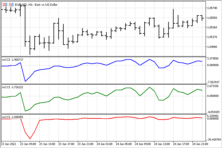
Now we can compare the behavior of different versions of the indicator. In some cases, the indicators look very similar.
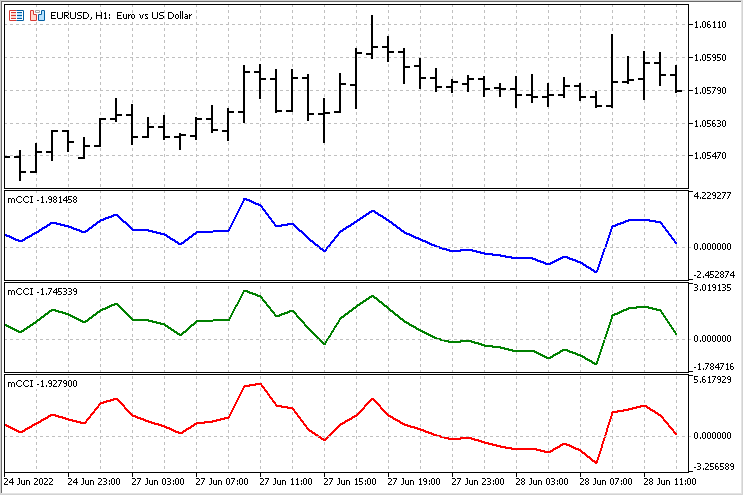
But there are also areas where the difference is quite noticeable.
A small Expert Advisor for comparing indicators
Visual comparisons are subjective and may lead to incorrect conclusions. We need more reliable basis for our conclusions. To evaluate all indicator version, let's write a simple Expert Advisor. Let's assign it the same rules for opening and closing positions, and compare the results. I will use the following rules — crossing a given level opens a position in one direction and closes positions in the opposite direction (if any).
EA parameters:
- TypeInd - indicator type (Classical, Square, Modern)
- iPeriod - indicator period
- iPrice - indicator price
- Level - level whose crossing is to be tracked. Its value of 150 corresponds to the level of 100 in the classic CCI.
To speed up the test, the indicator calculation algorithm has been moved inside the EA. The indicator values are calculated at the opening of a new bar. A Buy position is opened if the indicator value crosses the negative level value upwards. At the same time, Sell positions are closed. Sell positions are opened (and Buy positions are closed) if the indicator value crosses the positive level value downwards.
Test parameters:
EURUSD pair
H1 timeframe
time interval – the year of 2021
iPeriod = 14
iPrice = PRICE_TYPICAL
Level = 150
Balance curve options for all three cases are presented below.
TypeInd = Classical

TypeInd = Square

As we can see, applying the standard deviation has led to a decrease in the number of trades followed by a decrease in large losses.
TypeInd = Modern

The use of robust estimates has increased the number of trades, while the number of large losses has been reduced even more. This is a serious advantage for such an indicator version.
Regardless, the rules for opening and closing positions need serious improvements in all cases.
Indicator modification for estimating a trend
While carefully observing the CCI indicator (in any of its versions), I made an amazing discovery — it can take both positive and negative values. I do not know if this is worth the Nobel Prize, but MetaQuotes Ltd should establish its own award. I definitely deserve it. But enough kidding.
Positive indicator values are associated with an upward trend, while negative ones are related to a downward trend. Let's dwell on this in more detail. The general idea of the new indicator is as follows: we sum up the values of the CCI indicator from the moment a trend starts up to its end. Of course, we will compare this movement with the mean values. This way, we will be able to assess the duration of trend movements and their strength.
The version of calculations with robust estimates is to be used as a basis. The only difference is that we will accumulate the sum of the CCI indicator values after it overcomes the zero level. The value of this accumulated amount will be used as an output. The average amounts for uptrends and downtrends will be calculated separately for comparison. The general picture of this indicator looks as follows.
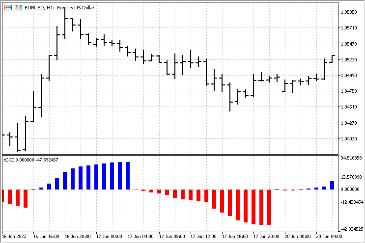
With this indicator, we can assess the beginning of a trend, its end and strength. The simplest strategy for this indicator may look like this - upon the trend completion, if the trend was above the average (the indicator crossed the corresponding level), we can expect the price to move in the opposite direction.
Conclusion
As we can see, a fresh look at technical indicators can be very useful. Not a single indicator is the final version - there is always the possibility of refinement and modification for specific strategies. Attached files:
- mCCI — indicator with three CCI versions
- EA CCI — trading EA to compare different CCI versions
- tCCI — indicator that calculates accumulated trend amounts.