
Third Generation Neural Networks: Deep Networks
Contents
- Second Generation Neural Networks
- 1.1. The Architecture of Connections
- 1.2. Main Types of Neural Networks
- 1.3. Training Methods
- 1.4. Disadvantages
- Deep Learning
- 2.1. Background
- 2.2. Autoencoders. Autoencoder and Restricted Boltzmann Machine. Differences and Peculiarities
- 2.3. Stacked Autoassociators Networks. Stackеd Autoencoder SAE, Stacked Restricted Boltzmann Machine (Stacked RBM)
- 2.4. Training of Deep Networks (DN). Stages. Peculiarities
- Practical Experiments
- 3.1. The R Language
- 3.2. Implementation Variations and Issues Addressed
- 3.3. Preparing data for the experiment
- 3.3.1. Source Data
- 3.3.2. Input Data (Predictors)
- 3.3.2.1. Welles Wilder's Directional Movement Index - ADX(HLC, n)
- 3.3.2.2. aroon(HL, n)
- 3.3.2.3. Commodity Channel Index - CCI(HLC, n)
- 3.3.2.4. chaikinVolatility (HLC, n)
- 3.3.2.5. Chande Momentum Oscillator - CMO(Med, n)
- 3.3.2.6. MACD oscillator
- 3.3.2.7. OsMA(Med,nFast, nSlow, nSig)
- 3.3.2.8. Relative Strength Index - RSI(Med,n)
- 3.3.2.9. Stochastic Oscillator - stoch(HLC, nFastK=14, nFastD=3, nSlowD=3)
- 3.3.2.10. Stochastic Momentum Index - SMI(HLC, n = 13, nFast = 2, nSlow = 25, nSig = 9)
- 3.3.2.11. Volatility (Yang and Zhang) - volatility(OHLC, n, calc="yang.zhang", N=96)
- 3.3.3. Output Data (Target)
- 3.3.4. Clearing Data
- 3.3.5. Training and Testing Sample Formation
- 3.3.6. Class Balancing
- 3.3.7. Preprocessing
- 3.4. Building, Training and Testing Models
- The Implementation (Indicator and Expert Advisor)
Introduction
This article is going to consider the main ideas of this subject such as Deep Learning and Deep Network without complex computations in layman’s terms.
Experiments with real data confirm (or don't) theoretical advantages of deep neural networks over shallow ones by metric definition and comparison. The task in hand is classification. We shall create an indicator and an Expert Advisor based on a deep neural network model and working in conjunction according to the client/server scheme and then test them.
The reader is presumed to have a fair idea of the basic concepts used in neural networks.
1. Second Generation Neural Networks
Neural networks are designed for addressing a wide range of problems connected with image processing.
Below is a list of problems typically solved by neural networks:
- Approximation of functions by a set of points (regression);
- Data classification by the specified set of classes;
- Data clustering with identification of previously unknown prototype classes;
- Information compression;
- Restoring lost data;
- Associative memory;
- Optimization, optimal control etc.
Out of the list above only "Classification" will be discussed in this article.
1.1. The Architecture of Connections
The way of information processing is greatly affected by absence or presence of feedback loops in the network. If there are no feedback loops between neurons (i.e. the network has a structure of sequential layers where every neuron receives information only from the previous layer), information processing in the network is unidirectional. An input signal is processed by a sequence of layers and the response is received in the number of tacts equal to the number of layers.
Presence of feedback loops can make the dynamic of a neural network (in this case called recurrent) unpredictable. Actually, a network can "loop forever" and never produce a response. At the same time, according to Turing, there is no algorithm for an arbitrary recurrent network to identify if its elements are going to get into equilibrium (the halting problem).
Generally speaking, the fact that neurons in recurrent networks participate in processing information many times, allows such networks to process information at a deeper level in different ways. In this case special measures should be taken so the network does not loop forever. For instance, use symmetric connections, like in a Hopfield network or forcefully limit the iterations number.
| Training type Connection type | With a "supervisor" | Without a "supervisor" |
|---|---|---|
| With no feedback loops | Multi-layered perceptrons (function approximation, classification) | Competitive network, self organizing maps (data compression, feature separation) |
| With feedback loops | Recurrent perceptron (time series prediction, on-line training) | Hopfield network (Associative memory, data clustering, optimization) |
Table 1. Neural network classification by connection type and training type
1.2. Main Types of Neural Networks
Having started with the perceptron, neural networks have gone a long way in their evolution. Today a large number of neural networks varying in structure and training methods are used.
The most famous are:
1.2.1. Multilayer Fully Connected Feedforward Networks MLP (Multilayer Perceptron)
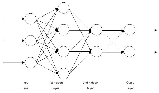
Fig. 1. Structure of a multilayer neural network
1.2.2. Jordan Networks are partially recurrent networks and similar to Elman networks.
It can be treated as a feedforward network with additional context neurons in the input layer.
These context neurons are fed by themselves (direct feedback) and from the input neurons. Context neurons preserve current state of the network. In a Jordan network the number of context and input neurons must be the same.
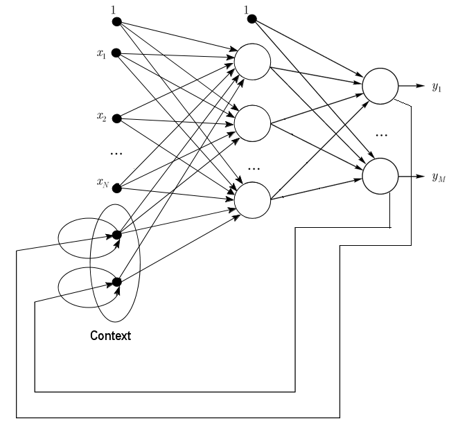
Fig. 2. Structure of a Jordan network
1.2.3. Elman Networks are partially recurrent networks and similar to Jordan networks. The difference between Elman and Jordan networks is that in an Elman network context neurons are not fed by output neurons, but by hidden ones. Besides, there is no direct feedback in context neurons.
In an Elman network the number of context and hidden neurons must be the same. The main advantage of Elman networks is that the number of context neurons is defined not by the number of outputs like in Jordan network but the number of hidden neurons, which makes the network more flexible. Hidden neurons can be easily added or taken away unlike the number of outputs.
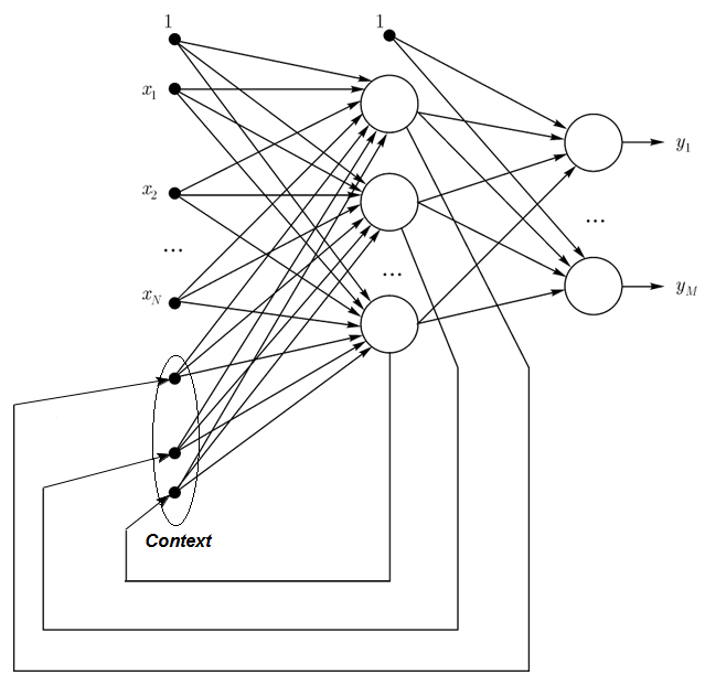
Fig. 3. Structure of an Elman network
1.2.4. Radial Basis Function Network (RBF) - is a feed-forward neural network that contains an intermediate (hidden) layer of radially symmetric neurons. Such a neuron converts the distance from a specified input vector to its correspondent center by some non-linear law commonly taken to be Gaussian.
The RBF networks have many advantages over multi layer feed forward networks. First of all, they emulate (not sure about the word) an arbitrary non linear function with only one intermediate layer, which saves the developer a necessity to decide on the number of layers. Then, parameters in the linear combination in the output layer can be optimized with the help of widely known methods of linear optimization. The latter work fast and do not have difficulties with local minimums that greatly interfere in backpropagation. That is the reason why the RBF network learns a lot faster than when using backpropagation.
Disadvantages of RBF: these networks have weak extrapolating characteristics and turn out to be cumbersome when the input vector is large.
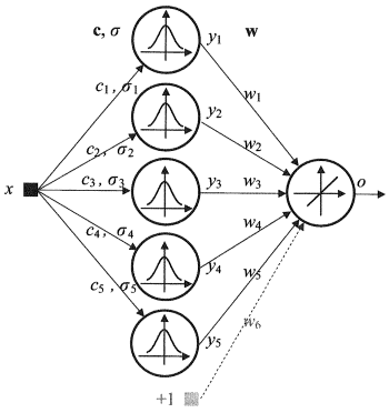
Fig. 4. Structure of an RBF
1.2.5. Dynamic Learning Vector Quantization, DLVQ Networks are very similar to the self organizing maps (SOM). Unlike SOM, DLVO are capable of supervised learning and lack a neighborhood relationship between the prototypes. Vector quantization has a wider use than clustering.
1.2.6. Hopfield Network is a fully connected network with a symmetrical connection matrix. During operation, dynamics of such networks converge to one of the equilibrium states. These equilibrium states are local minima of functionality known as energy of the network. Such a network can be used as a content-addressable associative memory system, as a filter and for addressing some optimization challenges.
Unlike many neural networks working till they receive a response in a certain number of tacts, Hopfield networks work till they reach the equilibrium state that is when the next state of a network is exactly the same as the previous one. In this case the initial state is an input pattern and in the equilibrium state the output image is received. Training a Hopfield network requires a training pattern to be presented at the input and output layers simultaneously.
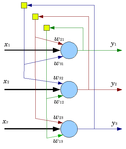
Fig. 5. Structure of a Hopfield network with three neurons
Despite appealing characteristics, a classical Hopfield network is far away from being ideal. It has limited memory, around 15% of the number of neurons in the network N, whereas systems of addressed memory can store up to 2N of different images, using N bits.
Besides, Hopfield networks are not capable of recognizing if the image is displaced or turned in relation to its initial stored position. These and other drawbacks define perception of a Hopfield network as a theoretical model convenient for study rather than a practical instrument for every day use.
Many others (Hemming recurrent network, Grossberg network, networks of adaptive resonance theory (ART-1, ART-2) etc) were not mentioned in this article as they are outside of the scope of our interest.
1.3. Training Methods
The ability to learn new things is the main characteristic of a human brain. In the case of artificial neural networks, learning is a process of configuring network architecture (the structure of connections between neurons) and weights of synaptic links (affecting coefficient signals) to obtain effective solution for the task in hand. Usually training of a neural network is performed on a data sample. A training process follows a certain algorithm and as it goes on, the network reaction to input signals should be improving.
There are three major learning paradigms: supervised, unsupervised and combined. In the first case the right answers for every input example are known and the weights are trying to minimize the error. Unsupervised learning allows categorizing samples through explaining the internal structure and nature of the data. In combined training both of the above approaches are used.
1.3.1. Main Rules of Neural Network Learning
There are four main learning rules based on the network architecture connected with them: error correction, Boltzmann's law, Hebb's rule and competitive learning.
1.3.1.1. Error Correction
Every input example has a specified desired output value (target value), which may mismatch a real (forecast) value. The error correction learning rule is using the difference between the target and the forecast values for direct adjustment of weights in order to decrease the error. Training is carried out only in the case of an erroneous outcome. This learning rule has numerous modifications.
1.3.1.2. Boltzmann's Rule
Boltzmann's rule is a stochastic learning rule by analogy with thermodynamic principles. This results in adjusting neurons' weight coefficients according to the desired probabilistic distribution. Learning Boltzmann's rule can be considered as an isolated case of correction by an error where an error means a correlation discrepancy of the states in two modes.
1.3.1.3. Hebb's Rule
Hebb's rule is the most famous algorithm of neural networks learning. The idea of this method is that if neurons on both sides of a synapse activate simultaneously and regularly, then the strength of the synaptic connection increases. An important peculiarity here is that synaptic weight change depends only on the activity of the neurons connected with this synapse. There are many variations of this rule that differ in peculiarities in synaptic weight modification.
1.3.1.4. Competitive Learning
Unlike Hebb's learning rule, where a number of output neurons can activate simultaneously, here output neurons compete against each other. An output neuron with maximal value of weighed sum is the "winner" and "the winner takes it all". Outputs of other output neurons are set to inactive. When learning, only the weights of the "winner" get modified targeting increasing proximity to the current input instance.
There are a lot of learning algorithms addressing different problems. Backpropagation, one of the most efficient modern algorithms, is one of them. The principle behind it is that synaptic weight change takes place with consideration for local gradient of the error function.
The difference between real and correct responses of a neural network evaluated at the output layer is back propagated - towards the stream of signals (Fig.5). This way every neuron can define contribution of its weight to the cumulative error of the network. The simplest learning rule is the steepest descent method, that is synaptic weight change proportionally to their contribution to the cumulative error.
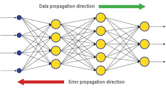
Fig. 6. The pattern of data and error diffusion in a network when learning through backpropagation
Surely, this type of neural network learning does not ensure the best learning result as there is always a possibility that the algorithm got into a local minimum. There are special techniques allowing to knock out the found solution from a local extreme point. If after a few applications of this technique the neural network has the same decision, then it can be concluded that the found solution is most likely to be optimal.
1.4. Disadvantages
- The main difficulty of using neural networks is the so called "curse of dimensionality". When input dimensions and the number of layers are increased, the complexity of a network and learning time are growing exponentially and the received result is not always optimal.
- Another difficulty of using neural networks is that traditional neural networks are unable to explain how they are solving tasks. In some application fields like medicine this explanation is more important than the result itself. Internal result representation is often so complex that it is impossible to analyze except simplest cases that are usually of no interest.
2. Deep Learning
Today theory and practice of machine learning is going through a "deep revolution", caused by successful implementation of the deep learning methods, representing third generation neural networks. Unlike classical second generation networks used in 80s-90s of the last century, new learning paradigms resolve a number of problems that restricted expansion and successful implementation of traditional neural networks.
Networks trained with deep learning algorithms did not simply excelled best alternative methods in accuracy but in some cases revealed rudiments of understanding sense of the input information. Image recognition and text information analysis are the brightest examples.
Today the most advanced industrial methods of computer vision and speech recognition are based on deep networks. Giants of the IT industry like Apple, Google, Facebook are employing researchers developing deep neural networks.
2.1. Background
A team of graduate students studying at the University of Toronto led by Professor Geoffrey E. Hinton won the top prize in a contest sponsored by Merck. Using a limited data set, describing the chemical structure of 15 molecules, G. Hinton's group managed to create and apply a special program system that defined which of those molecules was most likely to be an effective medicine.
The peculiarity of that work was that the developers used an artificial neural network based on deep learning. As a result that system managed to carry out calculations and research based on a very limited set of source data whereas training a neural network normally requires a significant amount of information put in the system.
Hinton's team achievement was particularly impressive because the team decided to enter the contest at the last minute. Added to that, the deep learning system was developed with no specific knowledge about how the molecules bind to their targets. Successful implementation of deep learning was yet another achievement in artificial intelligence development of the eventful 2012.
So in summer 2012, Jeff Dean and Andrew Y. Ng from Google presented a new image recognition system with accuracy rate 15,8%, where to train a cluster system of 16,000 nodes they used the ImageNet network containing a library of 14 million pictures of 20,000 different objects. Last year a program created by Swiss scientists outperformed a human in recognizing images of traffic signs. The winning program accurately identified 99.46 percent of the images in a set of 50,000; the top score in a group of 32 human participants was 99.22 percent, and the average for the humans was 98.84 percent. In October 2012, Richard F. Rashid, a coordinator of Microsoft scientific programs presented at a conference in Tianjin, China a technology of simultaneous translation from English into Mandarin accompanied by a simulation of his own voice.
All these technologies demonstrating a breakthrough in the field of artificial intelligence are based on the deep learning method to certain extent. The main contribution to the deep learning theory is being made by professor Hinton, a great-great grandson of George Boole, an English scientist, founder of the Boole algebra underlying contemporary computers.
The deep learning theory supplements ordinary methods of machine learning with special algorithms for the input information analysis at several presentation levels. The peculiarity of the new approach is that deep learning studies the subject till it finds enough informative presentation levels to account for all the factors that can influence parameters of the object in question.
This way, a neural network based on such an approach requires less input information for learning and a trained network is capable of analyzing information with a higher level of accuracy than usual neural networks. Professor Hinton and his colleagues state that their technology is especially good for searching peculiarities in multi-dimensional, well structured arrays of information.
The artificial intelligence technologies (AI), particularly deep learning, are widely used in different systems, including the intelligent personal assistant Apple Siri based on the Nuance Communications technologies and recognizing addresses in the Google Street View. Nevertheless, scientists are estimating success in this sphere very carefully as the history of creating an artificial intelligence is full of optimistic promises and disappointments.
In the 1960s, scientists believed that it would take only 10 years to create a fully featured artificial intelligence. Then in the 1980s, there was a wave of young companies offering a "ready-made artificial intelligence" followed by the "ice age" in this sphere, which lasted up to recently. Today wide computational capabilities available in cloud services provide a new level of powerful neural network implementation using new theoretical and algorithmic base.
It should be noted that neural networks, even third generation ones like convolutional neural networks, autoassociators, Boltzmann machines, have nothing in common with biological neurons except the name.
The new learning paradigm implements the learning idea in two stages. At the first stage, information about internal structure of the input data is extracted from a large array of unformatted data with autoassociator through layer-by-layer unsupervised training. Then, using this information in a multi-layer neural network, it goes through supervised training by known methods using formatted data. At the same time, the amount of unformatted data should be as large as possible. Formatted data can be a lot smaller in size. In our case it is not of immediate importance.
2.2. Autoencoders. Autoencoder and Restricted Boltzmann Machine. Differences and Peculiarities
2.2.1. Autoencoder
The first autoassociator (АА) was a Fukushima neocognitron.
Its structure is presented at Fig.7.

Fig. 7. A Fukushima neocognitron
The purpose of an autoassociator (АА) is to receive at the output as precise image of the input as possible.
There are two types of АА — generating and synthesizing. A restricted Boltzmann machine belongs to the first type and an autoencoder represents the second type.
An autoencoder is a neural network with one open layer. Using unsupervised learning algorithm and back propagation, it sets a target value equal to the input vector, i.e. y = x.
An example of an autoencoder is presented on Fig.8.
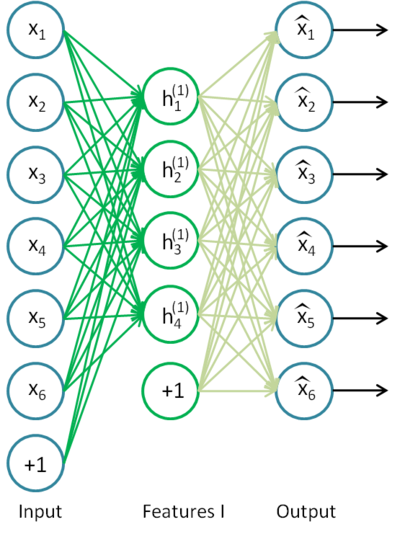
Fig. 8. An autoencoder structure
Autoencoder is trying to construct the function h(x)=x. In other words it is trying to find an approximation of a function ensuring that a neural network feedback is approximately equal to the values of input parameters. For the solution of the problem to be nontrivial, the number of neurons in the open layer must be less than the dimension of the input data (like on the picture).
It allows to compress data when the input signal gets passed to the network output. For example, if the input vector is a set of brightness levels of an image 10х10 pixels in size (100 characteristics), the number of neurons of the hidden layer is 50, the network is forced to learn to compress the image. The requirement h(x)=x means that based on the activation levels of fifty neurons of the hidden layer, the output layer is to restore 100 pixels of the initial image. Such compression is possible if there are hidden interconnections, characteristic correlation or any structure at all. This way an autoencoder operation reminds the principal component analysis method (PCA) in the sense that input data gets reduced.
Surprisingly, experiments conducted by Bengio et al. (2007), showed that when training with the stochastic gradient descent, nonlinear autocoding networks with the number of hidden neurons greater than the number of inputs (also called "superabundant") had useful presentation in the light of the conformance error of the network that took that presentation from the input.
Later, when the idea of sparsity appeared, a sparse autoencoder was widely used.
A sparse autoencoder is an autoencoder that has a number of hidden neurons significantly greater than the input dimension but they have a sparse activation. A sparse activation is when the number of inactive neurons in the hidden layer is significantly greater than the number of active ones. If we describe sparsity informally, then a neuron can be considered active if the value of its function is close to 1. If a sigmoid function is in use, then for the inactive neuron its value must be close to 0 (for the function of hyperbolic tangent the value should be close to -1).
There is a variation of an autoencoder called denoising autoencoder (Vincent et al., 2008). This is the same autoencoder but its training has some peculiarities. When training this network, "corrupted" data are input (some values are substituted with 0). At the same time, there is "correct" data to compare with the output data. This way an autoencoder can restore damaged data.
2.2.2. Restricted Boltzmann Machine, RBM.
We are not going to focus on the history of a restricted Boltzmann machine (RBM). All we need to know that it started with recurrent neural networks with feedback that were very difficult to train. Due to this learning difficulty, more restricted recurrent models appeared so simpler learning algorithms could be applied. A Hopfield neural network was one of such models. John Hopfield was the person who introduced the concept of the network energy having compared neural network dynamics with thermodynamics.
The next step on the way to an RBM was regular Boltzmann machines. They differ from a Hopfield network in having stochastic nature and its neurons are divided into two groups describing visible and hidden states (similar to a hidden Markov model). A restricted Boltzmann machine is different from a regular one in absence of connections between the neurons of one layer.
Fig. 9 represents an RBM structure.
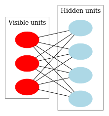
Fig. 9. An RBM structure
The peculiarity of this model is that in the present states of neurons of one group, the states of neurons of another group are going to be independent of one another. Now we can move on to some theory where this property has the key role.
Interpretation and objective
An RBM is interpreted similar to a hidden Markov model. We have a number of states that we can observe (visible neurons) and a number of hidden states that we cannot directly see (hidden neurons). We can come to a probability based conclusion about the hidden states relying on the states that we can observe. After such a model has been trained, we get an opportunity to draw conclusions regarding visible states knowing that the hidden ones are following Bayes' theorem. This allows generating data from the probability distribution used for training the model.
This way we can formulate the objective of training a model: the model parameters are to be adjusted the way so a restored vector from the initial state is closest to the original. A restored vector is a vector received by a probabilistic inference from hidden states, which in their turn, were received by a probabilistic inference from visible states, i.e. from the original vector.
Training algorithm is Contrastive Divergence CD-k
This algorithm was invented by Professor Hinton in 2002 and is remarkably simple. The main idea is that mathematical expectation values are substituted by defined values. Introduced is the idea of Gibbs sampling.
The CD-k looks like:
- The state of visible neurons is set equal to the input pattern;
- Probabilities of the hidden layer states are drawn;
- Each neuron of the hidden layer is assigned the state "1" with probability equal to its current state;
- Probabilities of the visible layer states are drawn based on the hidden layer;
- If the current iteration is less than k, then return to step 2;
- Probabilities of the hidden layer states are drawn;
In Hinton's lectures it looks like:
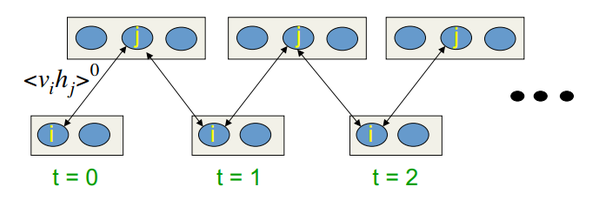
Fig.10. Algorithm of the CD-k learning
In other words, the longer we are doing sampling, the more precise the gradient is. Professor states that the result received for CD-1, i.e. only one sampling iteration, is already good.
2.3. Stacked Autoassociators Networks. Stackеd Autoencoder SAE, Stacked Restricted Boltzmann Machine (Stacked RBM)
For extracting high level abstractions from the input data set, autoassociators are combined into a network.
Fig. 11 represents a stackеd autoencoder structure and a neural network, which together represent a deep neural network with weights initialized by a stacked autoencoder
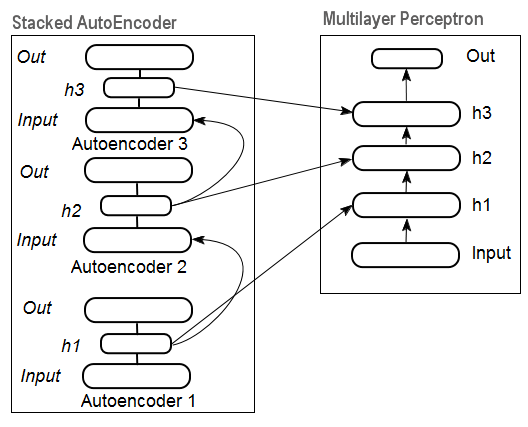
Fig. 11. Structure of a DN SAE
On Fig.12 there is a pattern of a stacked RBM (SRBM) and a neural network, which together represent a deep neural network with weights initialized by SRBM.
These illustrations of deep network structures emphasize the fact that the information gets extracted from bottom to top.
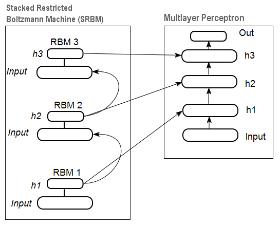
Fig. 12. Structure of a DN SRBM
2.4. Training of Deep Networks (DN). Stages. Peculiarities
Training deep networks comprises two stages. At the first stage, an autoassociator network (SAE or SRBM, depending on the DN type) receives unsupervised training on an unformatted data array. After that, hidden layer neurons of ordinary MLP get initialized by the hidden layer weights received after training. Fig. 11 and Fig. 12 represent a pattern of the learning and transfer processes. After training of the first АЕ/RBM, neuron weights of the hidden layer become inputs of the second one etc. This way, generalizing information about the structure (line, contour, patter etc) gets extracted from data.
The second stage is the time for fine-tuning of the MLP (supervised training) on formatted data set using well known methods. Practice proved that such initialization sets the neuron weights of the hidden layers of the MLP to the global minimum and the following fine-tuning takes a very short time.
Moreover, for deep networks with the number of layers greater than three, D. Hinton suggested that fine-tuning should be conducted in two stages. At the first stage only two upper layers should be trained and at the second one the rest of the network.
It should be mentioned that a SRBM has less stable results of unsupervised training than a SAE.
Note. Very often these terms are confused. A SRBM is identified with a deep belief network DBN. Despite the fact that a RBM derived from a DBN, these are totally different structures. A DBN is a multilayer neural network, with neuron weights of hidden layers initialized randomly by binary patterns.
3. Practical Experiments
Deep networks will be performed in R.
3.1. The R Language
History. R is a programming language and an environment for statistic computations and charting, developed in 1996 by New Zealand scientists Ross Ihaka and Robert Gentleman in Aokland University.
R is a GNU project that is a free software and its philosophy goes down to the following principles:
- freedom to launch programs for any purpose (freedom 0);
- freedom to learn how a program works and adapt it for own needs (freedom 1);
- freedom to distribute copies to help others (freedom 2);
- freedom to improve the program and let society benefit from the improvements.
In the historical perspective, R is an alternative for the implementation of S. The latter was developed by John Chambers and his colleagues in the Bell Labs company in 1976. Today, R is still being improved by R Development Core Team including John Chambers.
To repeat experiments, you will need to install R and Rstudio. Information on where to download and how can be found on the internet. If there are any questions, we can discuss them in the comments to the article.
Advantages of R:
- Today R is the standard in statistic computations.
- It is being developed and supported by the global scientific community of universities.
- Broad set of packages for all advanced fields of data mining. The time between a publication of the idea and its implementation in the R package is usually no longer that 2 weeks.
- And last but not the least, it is absolutely free. A famous developer of a free OS said once: "Programs are like sex - it is better when it is free".
3.2. Implementation Variations and Issues Addressed
There are two possible ways of implementation.
The first one involves using unique programs by John Hinton for Matlab. For that the "R.matlab" is required. This package has the writeMat() and readMat() methods for reading and writing the MAT files. It enables communication (code implementation, sending and receiving objects etc) from Matlab v6 and higher launched locally or on the remote host in the client-server link. Details can be found in the package description. This is the way for those who are comfortable using Matlab. I have not tried using this method but there is a possibility to link Matlab and MQL this way.
The second way of implementation is to use the R packages on this topic. We are going to explore it.
There are three packages I know are connected with the topic of this article:
"deepnet"is a simple package implementing the DN SAE and DN SRBM models. The length of the input data set at supervised and unsupervised learning is the same. Does not give an opportunity to perform fine-tuning of the system in two stages. Used for exploration and testing of the models at the beginning.
"darh" is an advanced and wide ranging package for modeling for DN SRBM. There is a model for DN SAE but I failed to launch it. This package is for experienced users, it allows creating and tuning a model of any complexity level. It is based on the unique programs by Hinton in the m language for MatLab.
"H2O" is an extensive package for training deep networks (not only them) on large data sets (>1 Гб) written in csv files.
In the below experiments we are going to use the "deepnet" package.
3.3. Preparing Input and Target Data for the Experiment
Today data mining has a certain work order:
- Selecting input data (studying, analysis, preliminary preparation, evaluation). Breaking data into the training, validation and test sets (samples);
- Training a model on the training data set and selecting a model/models on the validation one;
- Evaluation of the model/models quality on the test sample and defining optimal model parameters or the best model out of the set by certain measures;
- Letting the model/models to start the work.
The first stage is the most time consuming and very important for the end result. To be fair, this stage is not formalized and generally speaking it is nearly an art form. A lot depends on the experience of a researcher. However! Obtaining quantitative evaluations of the input data set for selecting the most important ones is very important. Automatic selection of the best variables for a certain model is even better in this case. R provides extensive functionality for meeting challenges at all stages.
Source data is not only very important but also has a lot of aspects to consider. It deserves a separate article. Since the goal of this article is to tell about a complex thing in very simple words, we will discuss important points but will not go into much detail.
3.3.1. Source Data
For our classification we need a set of independent (input) variables and a target variable. Since the main pronounced advantage of deep networks is their ability to quickly learn on large input samples, let us create a set of input data comprising 17 predictors (11 indicators). ZigZag has a role of the target variable. Download in the R environment vectors of the Open, High, Low, Close quotes 4000 bars deep. The way to do it is discussed below in the description of writing an indicator. At this stage it is not important. All further computations will be performed in R.
Construct a matrix out of 4 vectors, average price and size of the bar body. Turn it into a function:
pr.OHLC <- function (o, h, l, c)
{
  #Unite quote vectors into a matrix having previously expanded them
  #Indexing of time series of vectors in R starts with 1.
  #Direction of indexing is from old to new ones.
  price <- cbind(Open = rev(o), High = rev(h), Low = rev(l), Close = rev(c))
  Med <- (price[, 2] + price[, 3])/2
  CO <- price[, 4] - price[, 1]
  #add Med and CO to the matrix
  price <- cbind(price, Med, CO)
}
See the result (state at 08.10. 14 12:00)
> head(price)
        Open    High     Low   Close      Med     CO
[1,] 1.33848 1.33851 1.33824 1.33844 1.338375 -4e-05
[2,] 1.33843 1.33868 1.33842 1.33851 1.338550  8e-05
[3,] 1.33849 1.33862 1.33846 1.33859 1.338540  1e-04
[4,] 1.33858 1.33861 1.33856 1.33859 1.338585  1e-05
[5,] 1.33862 1.33868 1.33855 1.33855 1.338615 -7e-05
[6,] 1.33853 1.33856 1.33846 1.33855 1.338510  2e-05
3.3.2. Input Data (Predictors)
List the indicators. Indicators were selected randomly, with no preferences to gain maximal difference of input sizes.
Calculation of all indicators is performed using the "TTR" package containing numerous indicators.
3.3.2.1. Welles Wilder's Directional Movement Index - ADX(HLC, n) - 4 out (Dip, Din,DX, ADX)
Compute and see what it looks like on the first 200 bars:
> library(TTR)
> adx<-ADX(price, n = 16)
> plot.ts(head(adx, 200))
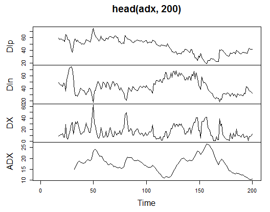
Fig. 13. Indicator Welles Wilder's Directional Movement Index - ADX(HLC, n)
> summary(adx)
      DIp             DIn                DX                 ADX
 Min.   :15.90   Min.   :  5.468   Min.   : 0.00831      Min.   : 5.482
 1st Qu.:41.21   1st Qu.: 33.599   1st Qu.: 8.05849      1st Qu.:14.046
 Median :47.36   Median : 43.216   Median :16.95423      Median :18.099
 Mean   :47.14   Mean   : 46.170   Mean   :19.73032      Mean   :19.609
 3rd Qu.:53.31   3rd Qu.: 55.315   3rd Qu.:27.97471      3rd Qu.:23.961
 Max.   :80.12   Max.   :199.251   Max.   :81.08751      Max.   :52.413
 NA's   :16      NA's   :16        NA's   :16            NA's   :31
In the beginning of the matrix there are 31 undefined values (NA). Then perform same calculations for all indicators without detailed explanations.
3.3.2.2. aroon(HL, n) - 1 out (oscillator)
Calculate and see the first 200 bars of only one variable "oscillator"
> ar<-aroon(price[ , c('High', 'Low')], n = 16)[ ,'oscillator']
> plot(head(ar, 200), t = "l")
> abline(h = 0)
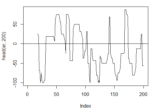
Fig. 14. Indicator aroon(HL, n)
> summary(ar)
   Min. 1st Qu.  Median    Mean 3rd Qu.    Max.    NA's
-100.00  -56.25  -18.75   -7.67   43.75  100.00      16
3.3.2.3. Commodity Channel Index - CCI(HLC, n) - 1 out
> cci<-CCI(price[ ,2:4], n = 16)
> plot.ts(head(cci, 200))
> abline(h = 0)
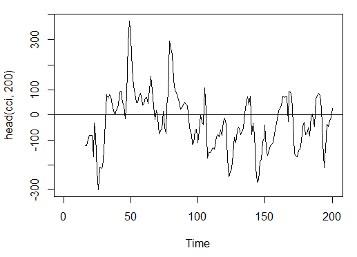
Fig. 15. Indicator Commodity Channel Index - CCI(HLC, n)
> summary(cci)
   Min. 1st Qu.  Median    Mean 3rd Qu.    Max.    NA's
-469.10  -90.95  -18.74  -14.03   66.91  388.20      15
3.3.2.4. Chaikin Volatility - chaikinVolatility (HLC, n) - 1 out
> chv<-chaikinVolatility(price[ , 2:4], n = 16)
> summary(chv)
    Min.  1st Qu.   Median     Mean  3rd Qu.     Max.     NA's
-0.67570 -0.29940  0.02085  0.12890  0.41580  5.15700       31
> plot(head(chv, 200), t = "l")
> abline(h = 0)
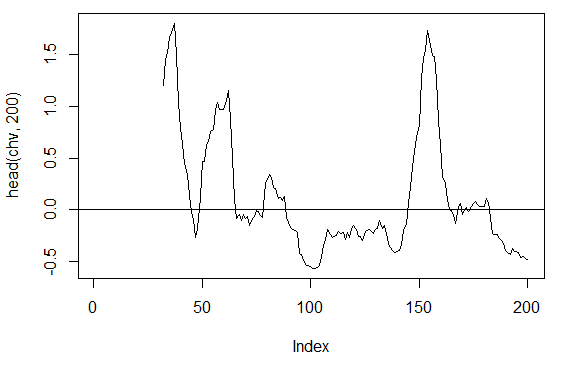
Fig. 16. Indicator chaikinVolatility (HLC, n)
3.3.2.5. Chande Momentum Oscillator - CMO(Med, n) - 1 out
> cmo<-CMO(price[ ,'Med'], n = 16)
> plot(head(cmo, 200), t = "l")
> abline(h = 0)
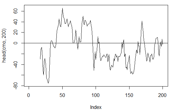
Fig. 17. Indicator Chande Momentum Oscillator - CMO(Med, n)
> summary(cmo)
   Min.    1st Qu.  Median    Mean 3rd Qu.    Max.    NA's
-97.670 -32.650  -5.400  -6.075  19.530  93.080      16
3.3.2.6. MACD oscillator - MACD(Med, nFast, nSlow, nSig) 1 out is used (macd)
> macd<-MACD(price[ ,'Med'], 12, 26, 9)[ ,'macd']
> plot(head(macd, 200), t = "l")
> abline(h = 0)
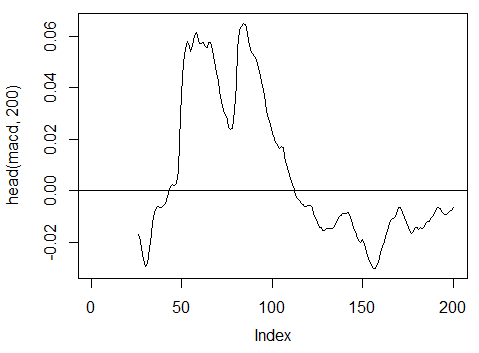
Fig. 18. Indicator MACD oscillator
> summary(macd)
     Min.   1st Qu.    Median      Mean   3rd Qu.      Max.      NA's
-0.346900 -0.025150 -0.005716 -0.011370  0.013790  0.088880      25
3.3.2.7. OsMA(Med,nFast, nSlow, nSig) – 1 out
> osma<-macd - MACD(price[ ,'Med'],12, 26, 9)[ ,'signal']
> plot(head(osma, 200), t = "l")
> abline(h = 0)
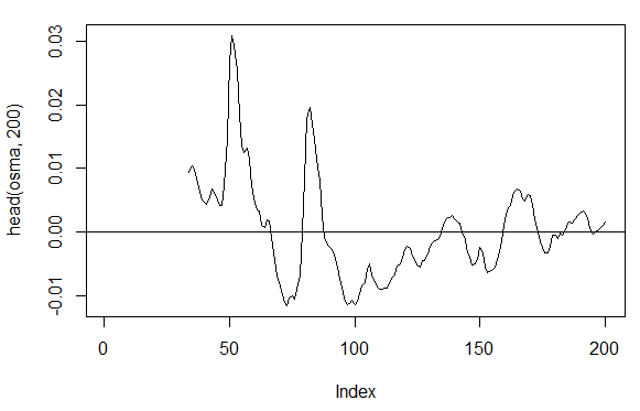
Fig. 19. Indicator OsMA(Med,nFast, nSlow, nSig)
> summary(osma)
    Min.  1st Qu.   Median     Mean  3rd Qu.     Max.     NA's
-0.10560 -0.00526  0.00034  0.00007  0.00646  0.05922       33
3.3.2.8. Relative Strength Index - RSI(Med,n) – 1 out
> rsi<-RSI(price[ ,'Med'], n = 16)
> plot(head(rsi, 200), t = "l")
> abline(h = 50)

Fig. 20. Indicator Relative Strength Index - RSI(Med,n)
> summary(rsi)
   Min. 1st Qu.  Median    Mean 3rd Qu.    Max.    NA's
   5.32   37.33   47.15   46.53   55.71   84.82      16
3.3.2.9. Stochastic Oscillator - stoch(HLC, nFastK=14, nFastD=3, nSlowD=3) - 3 out
> stoh<-stoch(price[ ,2:4], 14, 3, 3)
> plot.ts(head(stoh, 200))
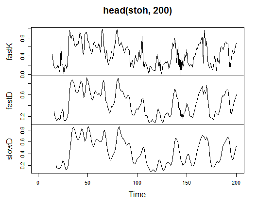
Fig. 21. Indicator Stochastic Oscillator - stoch(HLC, nFastK=14, nFastD=3, nSlowD=3)
> summary(stoh)
     fastK            fastD             slowD
 Min.   :0.0000   Min.   :0.01782   Min.   :0.02388
 1st Qu.:0.2250   1st Qu.:0.23948   1st Qu.:0.24873
 Median :0.4450   Median :0.44205   Median :0.44113
 Mean   :0.4622   Mean   :0.46212   Mean   :0.46207
 3rd Qu.:0.6842   3rd Qu.:0.67088   3rd Qu.:0.66709
 Max.   :1.0000   Max.   :0.99074   Max.   :0.97626
 NA's   :13       NA's   :15        NA's   :17
3.3.2.10. Stochastic Momentum Index - SMI(HLC, n = 13, nFast = 2, nSlow = 25, nSig = 9) — 2 out
> smi<-SMI(price[ ,2:4],n = 13, nFast = 2, nSlow = 25, nSig = 9)
> plot.ts(head(smi, 200))

Fig. 22. Indicator Stochastic Momentum Index - SMI(HLC, n = 13, nFast = 2, nSlow = 25, nSig = 9)
> summary(smi)
      SMI              signal
 Min.   :-82.185   Min.   :-78.470
 1st Qu.:-33.392   1st Qu.:-31.307
 Median : -9.320   Median : -8.839
 Mean   : -8.942   Mean   : -8.985
 3rd Qu.: 15.664   3rd Qu.: 14.069
 Max.   : 71.878   Max.   : 63.865
 NA's   :25        NA's   :33
3.3.2.11. Volatility (Yang and Zhang) - volatility(OHLC, n, calc="yang.zhang", N=96)- 1 out
> vol<-volatility(price[ ,1:4],n = 16,calc = "yang.zhang", N =96)
> plot.ts(head(vol, 200))
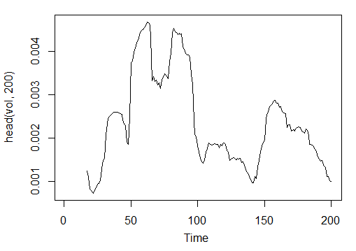
Fig. 23. Indicator Volatility (Yang and Zhang) - volatility(OHLC, n, calc="yang.zhang", N=96)
> summary(vol)
    Min.  1st Qu.   Median     Mean  3rd Qu.     Max.      NA's
0.000599 0.001858 0.002638 0.003127 0.004015 0.012840      16
So we have 17 variables from 11 indicators for EURUSD on the М15 timeframe for the OHLC sample 4000 bars deep.
Use them to form a matrix and write the above parameters in one function with one formal parameter р, which will be required for optimization.
Calculate the matrix of the input parameters using the formula:
In<-function(p = 16){
  adx<-ADX(price, n = p);
  ar<-aroon(price[ ,c('High', 'Low')], n=p)[ ,'oscillator'];
  cci<-CCI(price[ ,2:4], n = p);
  chv<-chaikinVolatility(price[ ,2:4], n = p);
  cmo<-CMO(price[ ,'Med'], n = p);
  macd<-MACD(price[ ,'Med'], 12, 26, 9)[ ,'macd'];
  osma<-macd - MACD(price[ ,'Med'],12, 26, 9)[ ,'signal'];
  rsi<-RSI(price[ ,'Med'], n = p);
  stoh<-stoch(price[ ,2:4],14, 3, 3);
  smi<-SMI(price[ ,2:4],n = p, nFast = 2, nSlow = 25, nSig = 9);
  vol<-volatility(price[ ,1:4],n = p,calc="yang.zhang", N=96);
  In<-cbind(adx, ar, cci, chv, cmo, macd, osma, rsi, stoh, smi, vol);
  return(In)
}
> X<-In()
> tail(X)
             DIp      DIn       DX      ADX   ar      cci       chv
[3995,] 46.49620 36.32411 12.28212 18.17544 25.0 168.0407 0.1835102
[3996,] 52.99009 31.61164 25.26952 18.61882 37.5 227.7030 0.3189822
[3997,] 58.11948 28.16241 34.72000 19.62515 37.5 145.2337 0.3448520
[3998,] 56.00323 30.48687 29.50206 20.24245 37.5 118.5831 0.3068059
[3999,] 55.96197 28.78737 32.06467 20.98134 37.5 116.5376 0.3517668
[4000,] 54.97777 26.85440 34.36713 21.81795 62.5 160.0767 0.6169701
             cmo         macd       osma      rsi     fastK
[3995,] 29.71342 -0.020870825 0.01666593 52.91932 0.8832685
[3996,] 41.89526 -0.009654368 0.02230591 61.49793 0.8833819
[3997,] 30.98237 -0.002051532 0.02392699 58.94513 0.7259475
[3998,] 33.84813  0.003454534 0.02354645 58.00549 0.7930029
[3999,] 38.84892  0.009590136 0.02374564 60.63806 0.8367347
[4000,] 54.71698  0.019303110 0.02676689 66.64815 0.9354120
            fastD     slowD        SMI    signal         vol
[3995,] 0.7773581 0.7735064 -35.095406 -47.27712 0.003643196
[3996,] 0.7691688 0.7761507 -26.482951 -43.11828 0.003858942
[3997,] 0.8308660 0.7924643 -19.699762 -38.43458 0.003920541
[3998,] 0.8007775 0.8002707 -13.141932 -33.37605 0.003916109
[3999,] 0.7852284 0.8056239  -6.569699 -28.01478 0.003999789
[4000,] 0.8550499 0.8136852   2.197810 -21.97226 0.004293766
Raw input data are prepared.
3.3.3. Output Data (Target)
Now we are going to form output (target data). As we mentioned before, we are going to use ZigZag.
We are going to use ZigZag with the channel width of 37 large points. ZigZag is going to be calculated by the average price. The indicator can be calculate by the HL prices, however the average price is preferable as the indicator is more stable in this case. Having extracted the signal (0 - Buy, 1 -Sell), convert it into an input matrix, which assumes the network model.
Write a function:
Out<-function(ch=0.0037){
  # ZigZag has values on each bar and not only in the points
  zz<-ZigZag(price[ ,'Med'], change = ch, percent = F, retrace = F, lastExtreme = T);
  n<-1:length(zz);
  # On the last bars substitute the undefined values for the last known ones
  for(i in n) { if(is.na(zz[i])) zz[i] = zz[i-1];}
  #Define the speed of ZigZag changes and move one bar forward
  dz<-c(diff(zz), NA);
  #If the speed >0 - signal = 0(Buy), if <0, signal = 1 (Sell) otherwise NA
  sig<-ifelse(dz>0, 0, if else(dz<0, 1, NA));
  return(sig);
}
Calculate signals.
> Y<-Out()
> table(Y)
Y
   0    1
1567 2423
Class ratio is unbalanced. Number of examples of one class is greater than the other one. All models of the classification are unfriendly towards such sets.
When separating data into training and test samples, we will rectify this situation.
3.3.4. Clearing Data
Clear our data sets from undefined data. Clearing in this case implies a wider round of tasks. It includes clearing "virtually zero variables" and high correlated ones as well as some other tasks we are not going to discuss here.
Write a function and clear the data
Clearing<-function(x, y){
  dt<-cbind(x,y);
  n<-ncol(dt)
  dt<-na.omit(dt)
  return(dt);
}
> dt<-Clearing(X,Y); nrow(dt)
[1] 3957
The matrix has become 43 bars shorter.
3.3.5. Training and Testing Sample Formation
There are several ways of breaking the source data into the training and test samples. We are going to employ regular random division of the source data into the train and test one in proportion 8/10. It is important that the samples are stratified, which means that the ratio of the class instances in train and test samples must correspond to the class ratio in the source data set. It would also be beneficial to rectify class inequality in the source data set. There are two ways of doing it - either leveling by the greater or by the smaller class. As we require more examples, we are going to level by the greater class "1". In this case we are going to use the "caret" package.
Let us form a new balanced set where the number of instances of both classes are the same and are equal to the greater one.
3.3.6. Class Balancing
Below is the function that levels the number of classes by the greater side (if the divergence is greater than 15%) and returns a balanced matrix
Balancing<-function(DT){
  #Calculate a table with a number of classes
  cl<-table(DT[ ,ncol(DT)]);
  #If the divergence is less than 15%, return the initial matrix
  if(max(cl)/min(cl)<= 1.15) return(DT)
  #Otherwise level by the greater side
  DT<-if(max(cl)/min(cl)> 1.15){
         upSample(x = DT[ ,-ncol(DT)],y = as.factor(DT[ , ncol(DT)]), yname = "Y")
        }
  #Convert у (factor) into a number
  DT$Y<-as.numeric(DT$Y)
  #Recode у from 1,2 into 0,1
  DT$Y<-ifelse(DT$Y == 1, 0, 1)
  #Convert dataframe to matrix
  DT<-as.matrix(DT)
  return(DT);
}
Explanation. In the first string calculate the number of instances of each class (vector, with the dimension equal to the number of classes).
Find the ratio of the greater vector to the smaller one and if it is less than the set threshold one, exit. If the ratio is greater, then calculate the function, having put in х and y separately. Y must be previously converted into a factor.
This is the requirement to the formal parameters of the upSample() function. Since we do not need the target variable as a factor, we convert it back into a numeric one with values 0 and 1. Please note that when we convert a numeric variable (0,1) into a factor, we receive text variables "0" and "1". At the reversed conversion into numeric variables, we get 1 and 2 (!). We replace them with 0 and 1. Our data set gets converted from the "data frame" to the class "matrix". Calculate it:
dt.b<-Balancing(dt)
x<-dt.b[ ,-ncol(dt.b)]
y<-dt.b[ , ncol(dt.b)]
This way we have the source dt data set (input and output) and the balanced set dt.b.
Divide it into the train and test samples
Obtain the indices of the train and test samples from the "rminer" package using the holdout() function.
> library('rminer')
> t<-holdout(y, ratio = 8/10, mode = "random")
The t object is a list containing indices of the training (t$tr) and the test (t$ts) data set. The received sets are stratified.
3.3.7. Preprocessing
Our input data source contains variables with different value ranges. Essentially, deep networks are regular networks with a peculiar way of initializing weights.
Neural networks can receive the input variables in the range (-1; 1) or (0, 1). Normalize the input variables into the range of [-1, 1].
For that use the preProcess() function from the "caret" package. Please note that the parameters of preprocessing are to be calculated on the training data set and save them for further preprocessing of the test data set and newly input data.
> spSign<-preProcess(x[t$tr, ], method = "spatialSign")
> x.tr<-predict(spSign, x[t$tr, ])
> x.ts<-predict(spSign, x[t$ts, ])
Now we have everything for building, training and testing a deep neural network.
3.4. Building, Training and Testing Models
We are going to build and train the DN SAE model. The formula of the model and description of the variables:
sae.dnn.train(x, y, hidden = c(10), activationfun = "sigm", learningrate = 0.8, momentum = 0.5, learningrate_scale = 1, output = "sigm", sae_output = "linear",
  numepochs = 3, batchsize = 100, hidden_dropout = 0, visible_dropout = 0)
where:
- х is a matrix of input data;
- y is a vector or matrix of target variables;
- hidden is a vector with a number of neurons in every hidden layer. By default с(10);
- activationfun is a function of activating hidden neurons. Can be "sigm", "linear", "tanh". By default "sigm";
- learningrate is a training level for the gradient descent. By default = 0.8;
- momentum is a momentum for the gradient descent. By default = 0.5;
- learningrate_scale training level can be multiplied by this value after every iteration. By default =1.0;
- numepochs is a number of iterations for training. By default =3;
- batchsize is the size of small amount of data being trained. By default =100;
- output is the activation function for output neurons can be "sigm", "linear", "softmax". By default "sigm";
- sae_output is the activation function of output neurons of SAE, can be "sigm", "linear", "softmax". By default "linear";
- hidden_dropout is a deletable part for hidden layers. By default =0;
- visible_dropout is a deletable part of the visible (input) layer. By default =0.
We are going to create a model with the following dimensions (17, 100, 100, 100, 1), train it, note the time of learning and observe the forecast.
> system.time(SAE<-sae.dnn.train(x= x.tr, y= y[t$tr], hidden=c(100,100,100), activationfun = "tanh", learningrate = 0.6, momentum = 0.5, learningrate_scale = 1.0, output = "sigm", sae_output = "linear", numepochs = 10, batchsize = 100, hidden_dropout = 0, visible_dropout = 0))
begin to train sae ......
training layer 1 autoencoder ...
training layer 2 autoencoder ...
training layer 3 autoencoder ...
sae has been trained.
begin to train deep nn ......
deep nn has been trained.
   user  system elapsed
  12.92    0.00   13.09
As we can see, it happens in two stages. At first autoencoder gets trained layer by layer and then the neural network.
The small number of training times and immense number of hidden neurons in the three layers were set on purpose. The whole process took 13 seconds!
Let us evaluate forecasts on the test set of predictors.
> pr.sae<-nn.predict(SAE, x.ts);
> summary(pr.sae)
       V1
 Min.   :0.2649
 1st Qu.:0.2649
 Median :0.5881
 Mean   :0.5116
 3rd Qu.:0.7410
 Max.   :0.7410
Convert into the levels 0,1 and calculate measurements
> pr<-ifelse(pr.sae>mean(pr.sae), 1, 0)
> confusionMatrix(y[t$ts], pr)
Confusion Matrix and Statistics

          Reference
Prediction   0   1
         0 316 128
         1 134 378

               Accuracy : 0.7259
                 95% CI : (0.6965, 0.754)
    No Information Rate : 0.5293
    P-Value [Acc > NIR] : <2e-16

                  Kappa : 0.4496
 Mcnemar's Test P-Value : 0.7574

            Sensitivity : 0.7022
            Specificity : 0.7470
         Pos Pred Value : 0.7117
         Neg Pred Value : 0.7383
             Prevalence : 0.4707
         Detection Rate : 0.3305
   Detection Prevalence : 0.4644
      Balanced Accuracy : 0.7246

       'Positive' Class : 0
This is not an outstanding coefficient. We are more interested in the profit that we are going to make using these signals, not the coefficient. Check it on the last 500 bars (approximately a week). We are going to receive signals on the last 500 sequential bars from our trained network.
Normalize the last 500 bars of input data, receive forecasts from the trained neural network and convert them into signals -1= (Sell) and 1 = (Buy)
> new.x<-predict(spSign,tail(dt[ ,-ncol(dt)], 500))
> pr.sae1<-nn.predict(SAE, new.x)
> pr.sig<-ifelse(pr.sae1>mean(pr.sae1), -1, 1)
> table(pr.sig)
pr.sig
 -1   1
235 265
> new.y<-ifelse(tail(dt[  , ncol(dt)], 500) == 0, 1, -1)
> table(new.y)
new.y
 -1   1
201 299
> cm1<-confusionMatrix(new.y, pr.sig)
> cm1
Confusion Matrix and Statistics

          Reference
Prediction  -1   1
        -1 160  41
        1   75 224

               Accuracy : 0.768
                 95% CI : (0.7285, 0.8043)
    No Information Rate : 0.53
    P-Value [Acc > NIR] : < 2.2e-16

                  Kappa : 0.5305
 Mcnemar's Test P-Value : 0.002184

            Sensitivity : 0.6809
            Specificity : 0.8453
         Pos Pred Value : 0.7960
         Neg Pred Value : 0.7492
             Prevalence : 0.4700
         Detection Rate : 0.3200
   Detection Prevalence : 0.4020
      Balanced Accuracy : 0.7631

       'Positive' Class : -1
The Accuracy coefficient is not bad, though we are more interested in the profit, not the coefficient.
Test the profit for the last 500 bars using our predicted signals and get the balance curve:
> bal<-cumsum(tail(price[ , 'CO'], 500) * pr.sig)
> plot(bal, t = "l")
> abline(h = 0)
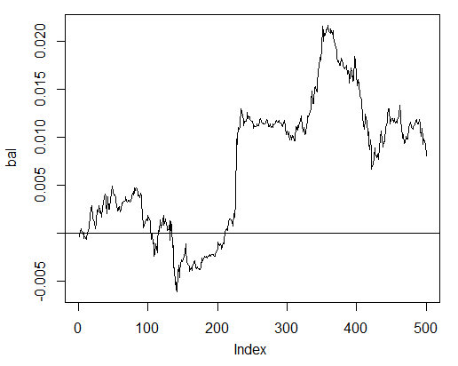
Fig. 24. Balance on the last 500 bars by the neural network signals
The balance was calculated without taking into consideration spread, slippage and other realities of a live market.
Now compare with the balance that would have been obtained from the ideal signals of ZZ. The red line is the balance by the neural network signals:
> bal.zz<-cumsum(tail(price[ , 'CO'], 500) * new.y)
> plot(bal.zz,  t = "l")
> lines(bal,  col = 2)
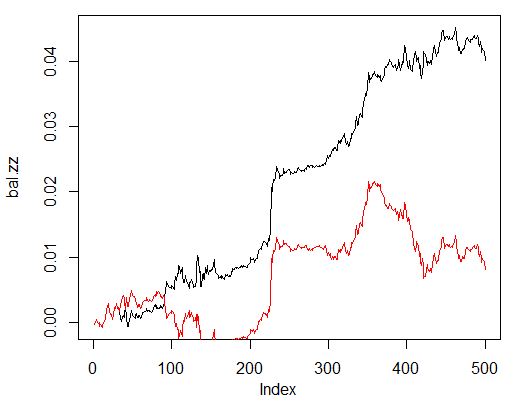
Fig. 25. Balance on the last 500 bars by the neural network signals and the ZigZag signals
There is potential for improvement.
Write two functions to facilitate two helper functions Estimation() and Testing(). The first will generate coefficients Accuracy/Err and the second one balance Bal/BalZZ.
It allows to obtain a result straight away changing some network parameters and see what parameters influence the quality of the network.
Having written a fitness function, optimal network parameters can be found using evolutionary (genetic) algorithm without any disruptions for the trading process. We are not going to dedicate time to it in this article and will consider it in detail some other time.
Below is the function Estimation() calculating coefficients Err/Accuracy:
Estimation<-function(X, Y, r = 8/10, m = "random", norm = "spatialSign",
                     h = c(10), act = "tanh", LR = 0.8, Mom = 0.5,
                     out = "sigm", sae = "linear", Ep = 10, Bs = 50,
                     CM=F){
  #Indices of the training and test data set
  t<-holdout(Y, ratio = r, mode = m)
  #Parameters of preprocessing
  prepr<-preProcess(X[t$tr,  ], method = norm)
  #Divide into train and test data sets with preprocessing
  x.tr<-predict(prepr, X[t$tr,  ])
  x.ts<-predict(prepr, X[t$ts,  ])
  y.tr<- Y[t$tr]; y.ts<- Y[t$ts]
  #Train the model
  SAE<-sae.dnn.train(x = x.tr , y = y.tr , hidden = h,
                     activationfun = act,
                     learningrate = LR, momentum = Mom,
                      output = out, sae_output = sae,
                     numepochs = Ep, batchsize = Bs)
  #Obtain a forecast on the test data set
  pr.sae<-nn.predict(SAE, x.ts)
  #Recode it into signals 1,0
  pr<-ifelse(pr.sae>mean(pr.sae), 1, 0)
  #Calculate the Accuracy coefficient or classification error
  if(CM) err<-unname(confusionMatrix(y.ts, pr)$overall[1])
  if(!CM) err<-nn.test(SAE, x.ts, y.ts, mean(pr.sae))
  return(err)
}
Formal parameters:
- X – matrix of input raw predictors;
- Y – vector of the target variable;
- r – ratio train/test;
- m – sample formation mode (random or consequent);
- norm – mode of input parameters normalizing ([ -1, 1]= "spatialSign";[0, 1]="range");
- h – vector with a number of neurons in the hidden layers;
- act – activation function of hidden neurons;
- LR – training level;
- Мом — momentum;
- out – activation function of the output layer;
- sae – activation function of the autoencoder;
- Ep – number of the training epochs;
- Bs – size of the small sample;
- СM– Boolean variable , if TRUE print Accuracy. Else Err.
As an example we are going to calculate the classification error on the unbalanced data set dt by the network with three hidden layers each containing 30 neurons:
> Err<-Estimation(X = dt[ ,-ncol(dt)], Y = dt[ ,ncol(dt)], h=c(30, 30, 30), LR= 0.7)
begin to train sae ......
training layer 1 autoencoder ...
training layer 2 autoencoder ...
training layer 3 autoencoder ...
sae has been trained.
begin to train deep nn ......
deep nn has been trained.
> Err
[1] 0.1376263
The function Testing() calculates balance by the forecast signals or by the ideal ones (ZigZag):
Testing<-function(dt1, dt2, r=8/10, m = "random", norm = "spatialSign",
                     h = c(10), act = "tanh", LR = 0.8, Mom = 0.5,
                     out = "sigm", sae = "linear", Ep = 10, Bs=50,
                     pr = T, bar = 500){
  X<-dt1[  ,-ncol(dt1)]
  Y<-dt1[  ,ncol(dt1)]
  t<-holdout(Y,  ratio = r,  mode = m)
  prepr<-preProcess(X[t$tr,  ], method = norm)
  x.tr<-predict(prepr, X[t$tr,  ])
  y.tr<- Y[t$tr];
  SAE<-sae.dnn.train(x = x.tr , y = y.tr , hidden = h,
                     activationfun = act,
                     learningrate = LR, momentum = Mom,
                     output = out, sae_output = sae,
                     numepochs = Ep, batchsize = Bs)
  X<-dt2[ ,-ncol(dt2)]
  Y<-dt2[ ,ncol(dt2)]
  x.ts<-predict(prepr, tail(X, bar))
  y.ts<-tail(Y, bar)
  pr.sae<-nn.predict(SAE, x.ts)
  sig<-ifelse(pr.sae>mean(pr.sae), -1, 1)
  sig.zz<-ifelse(y.ts == 0, 1,-1 )
  bal<-cumsum(tail(price[  ,'CO'], bar) * sig)
  bal.zz<-cumsum(tail(price[  ,'CO'], bar) * sig.zz)
  if(pr) return(bal)
  if(!pr) return(bal.zz)
}
Formal parameters:
- dt1 – matrix of the input and target variable used for training the network;
- dt2 - matrix of the input and target variables used for testing the network;
- pr – Boolean variable, if TRUE print the balance by the forecast signals, otherwise by ZigZag;
- bar - the number of the last bars to use for calculating balance.
Calculate balance on the last 500 bars of our data set dt when training on the balanced data set dt.b by the neural network with the same parameters as above:
> Bal<-Testing(dt.b, dt, h=c(30, 30, 30), LR= 0.7)
begin to train sae ......
training layer 1 autoencoder ...
training layer 2 autoencoder ...
training layer 3 autoencoder ...
sae has been trained.
begin to train deep nn ......
deep nn has been trained.
> plot(Bal, t = "l")
> abline(h = 0)
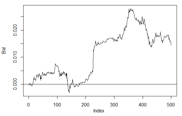
Fig. 26. Balance on the last 500 bars by the neural network signals h(30,30,30)
If we compare the result with the previously obtained balance then we can see a significant improvement. This is not the most interesting point here though.
If we take a look at the price plot on the last 500 bars, then we can see what parts of it were best accepted by our network (150-350 bars).
> plot(tail(price[  ,'Close'], 500), t = "l")
> abline(v = c(150,350), col=2)
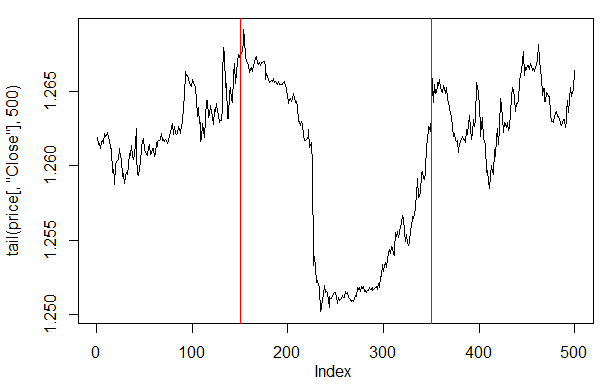
Fig. 27. Plot of the Close price on the last 500 bars
Note: When decoding the forecast outputs, we used a simplified version greater/less than the average, though other versions can be used.
If the values are greater than 0.6 or less than 0.4, the unstable segment of 0.4-0.6 gets cut off. More precise class boundaries can be obtained at calibration. This is going to be discussed later.
Our function Testing() is going to be changed a little if an additional parameter dec is going to be introduced. This will allow us to select a way to decode ("mean" or "60/40") and check on the predicted values what impact it is going to have on the balance.
Testing.1<-function(dt1, dt2, r = 8/10, m = "random", norm = "spatialSign",
                     h = c(10), act = "tanh", LR = 0.8, Mom = 0.5,
                     out = "sigm", sae = "linear", Ep = 10, Bs = 50,
                     pr = T, bar = 500, dec=1){
  X<-dt1[ ,-ncol(dt1)]
  Y<-dt1[ ,ncol(dt1)]
  t<-holdout(Y, ratio = r, mode = m)
  prepr<-preProcess(X[t$tr, ], method = norm)
  x.tr<-predict(prepr, X[t$tr, ])
  y.tr<- Y[t$tr];
  SAE<-sae.dnn.train(x = x.tr , y = y.tr , hidden = h,
                     activationfun = act,
                     learningrate = LR, momentum = Mom,
                     output = out, sae_output = sae,
                     numepochs = Ep, batchsize = Bs)
  X<-dt2[ ,-ncol(dt2)]
  Y<-dt2[ ,ncol(dt2)]
  x.ts<-predict(prepr, tail(X, bar))
  y.ts<-tail(Y, bar)
  pr.sae<-nn.predict(SAE, x.ts)
  #Variant +/- mean
  if(dec == 1) sig<-ifelse(pr.sae>mean(pr.sae), -1, 1)
  #Variant 60/40
  if(dec == 2) sig<-ifelse(pr.sae>0.6, -1, ifelse(pr.sae<0.4, 1, 0))
  sig.zz<-ifelse(y.ts == 0, 1,-1 )
  bal<-cumsum(tail(price[  ,'CO'], bar) * sig)
  bal.zz<-cumsum(tail(price[  ,'CO'], bar) * sig.zz)
  if(pr) return(bal)
  if(!pr) return(bal.zz)
}
Calculate and assess the balance with the first and the second ways of decoding.
In order the results to repeat, set pseudorandom number generator in the same position.
> set.seed<-1245
> Bal1<-Testing.1(dt.b, dt, h = c(30, 30, 30), LR = 0.7, dec = 1)
begin to train sae ......
training layer 1 autoencoder ...
training layer 2 autoencoder ...
training layer 3 autoencoder ...
sae has been trained.
begin to train deep nn ......
deep nn has been trained.
> set.seed<-1245
> Bal2<-Testing.1(dt.b, dt, h = c(30, 30, 30), LR = 0.7, dec = 2)
begin to train sae ......
training layer 1 autoencoder ...
training layer 2 autoencoder ...
training layer 3 autoencoder ...
sae has been trained.
begin to train deep nn ......
deep nn has been trained.
> plot(Bal2, t = "l")
> lines(Bal1, col = 2)
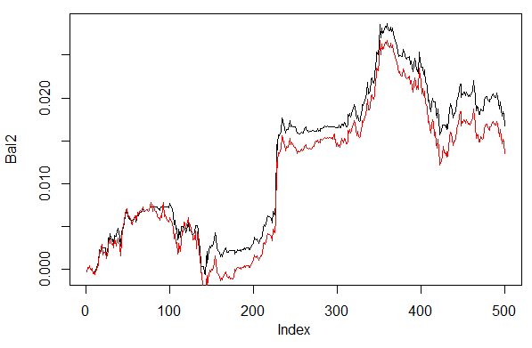
Fig. 28. Balance for the last 500 bars by the neural network signals with different ways of decoding forecasts
Clearly, balance by the second way 60/40 looks better. There is space for improvement in this aspect too.
Here is the last thing to check. In theory, an ensemble of several neural networks gives a better and more stable result. We are going to test an ensemble consisting of several networks, which are trained on the same samples though they can be trained on independent samples. The result of the ensemble's forecast is a simple average of the forecasts of all the networks. There are other more complex ways of averaging.
We are going to improve our function Testing() by adding one more parameter — ans=1 specifying the number of the networks in the ensemble.
3.4.1. Parallel Calculations
Since computations by several independent models can easily be paralleled, we are going to use the opportunity provided by the R language and create a cluster consisting of a several processor cores or computers of a local networks irrespective to what operating systems these computers have.
For that we need the "foreach" and the "doParallel" packages. Below is a very simple function that will launch a cluster for all the cores of our processor.
library(doParallel)
library(foreach)
puskCluster<-function(){
  cores<-detectCores()
  cl<-makePSOCKcluster(cores)
  registerDoParallel(cl)
  clusterSetRNGStream(cl)
 return(cl)
}
Several points are clarified below. In the first two strings we load necessary libraries. They need to be previously installed on your computer. Then we define how many cores there are in the processor, create a cluster, register a package for parallel computations, install an independent pseudorandom number generator in every stream of calculations and return the cluster handle. Quality of the pseudorandom number generator for computations of every model is extremely important though this is a separate topic.
After the cluster has been launched and all required computations have been made, we must remember to stop it:
cl<-puskCluster()
stopCluster(cl)
Parallel computations are going to be performed by the following formula from the "foreach" package:
SAE<-foreach(times(ans), .packages = "deepnet") %dopar%
                sae.dnn.train(x = x.tr , y = y.tr , hidden = h,
                        activationfun = act,
                        learningrate = LR, momentum = Mom,
                        output = out, sae_output = sae,
                        numepochs = Ep, batchsize = Bs)
where times(ans) is a number of networks that we want to obtain and .packages points to the package to take the calculated function.
The result has a form of a list and contains the number of trained networks we need.
Then we require the forecast from every network and calculate the average.
pr.sae<-(foreach(i = 1:ans, .combine = "+") %do% nn.predict(SAE[[i]], x.ts))/ans
Here i is a vector of the trained network indices,.combine="+" specifies what form the returned predicts in all neural networks are supposed to be returned in. In this case we required to return a sum and perform these computations sequentially, not in a parallel way (operator %do%). The obtained sum is going to be divided by the number of the neural networks and it will be the end result. This is nice and simple.
Calculate balance obtained from ensembles consisting of 3 and 4 neural networks with the same parameters that the ones above and using the decoding way 60/40. Compare with the results on one neural network. To evaluate effectiveness of parallel computations, increase the number of epochs to 300 and time the process of obtaining the forecast.
1. One neural network:
> system.time(Bal21<-Testing.1(dt.b, dt, h = c(30, 30, 30), LR = 0.7, dec = 2, Ep=300))
begin to train sae ......
training layer 1 autoencoder ...
####loss on step 10000 is : 0.000057
####loss on step 20000 is : 0.000043
training layer 2 autoencoder ...
####loss on step 10000 is : 0.000081
####loss on step 20000 is : 0.000086
training layer 3 autoencoder ...
####loss on step 10000 is : 0.000072
####loss on step 20000 is : 0.000066
sae has been trained.
begin to train deep nn ......
####loss on step 10000 is : 0.069451
####loss on step 20000 is : 0.079629
deep nn has been trained.
   user  system elapsed
 115.78    0.00  116.96
> plot(Bal21, t = "l")
> abline(h = 0)
2. Ensemble of 3 neural networks:
> system.time(Bal41<-Testing.2(dt.b, dt, h = c(30, 30, 30), LR = 0.7, Ep=300, dec = 2, ans=3))
   user  system elapsed
   0.22    0.06  233.64
> lines(Bal41, col=4)
3. Ensemble of 4 neural networks:
> system.time(Bal44<-Testing.2(dt.b, dt, h = c(30, 30, 30), LR = 0.7, Ep=300, dec = 2, ans=4))
   user  system elapsed
   0.13    0.03  247.86
> lines(Bal44, col=2)
Execution time at parallel computation is optimal if the number of streams is multiple to the number of cores. I have used 2 cores.
Saying that, there is no significant advantages in the balance. On the chart below, the blue plot denotes 3 networks, the red one - 4 networks and the black one - one network.
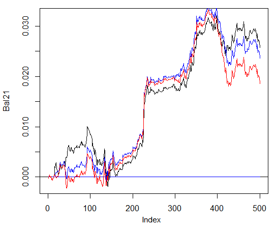
Fig. 29. Balance on the last 500 bars by the signals of the ensembles consisting of 3 and 4 neural networks and one network
In general, the result depends on many parameters, starting from input and output data, the way of their normalizing, the number of hidden layers and the number of neurons in those layers, training level, the number of training epochs and many others.
Last three examples. Calculate balance on the last 1000 bars with three neural networks with different numbers of hidden neurons in three hidden layers.
> system.time(Bal0<-Testing.1(dt.b, dt, h = c(30, 30, 30), LR = 0.7, dec = 2, Ep=300, bar=1000))
begin to train sae ......
training layer 1 autoencoder ...
####loss on step 10000 is : 0.000054
####loss on step 20000 is : 0.000044
training layer 2 autoencoder ...
####loss on step 10000 is : 0.000078
####loss on step 20000 is : 0.000079
training layer 3 autoencoder ...
####loss on step 10000 is : 0.000090
####loss on step 20000 is : 0.000072
sae has been trained.
begin to train deep nn ......
####loss on step 10000 is : 0.072633
####loss on step 20000 is : 0.057917
deep nn has been trained.
   user  system elapsed
 116.09    0.02  116.26
> max(Bal0)
[1] 0.04725
> plot(Bal0, t="l")
> tail(Bal0,1)
[1] 0.03514
Maximum profit is 472 points, on the last bar 351 points. On the chart it is drawn in black.
> system.time(Bal0<-Testing.1(dt.b, dt, h = c(13, 8, 5), LR = 0.7, dec = 2, Ep=300, bar=1000))
begin to train sae ......
training layer 1 autoencoder ...
####loss on step 10000 is : 0.005217
####loss on step 20000 is : 0.004846
training layer 2 autoencoder ...
####loss on step 10000 is : 0.051324
####loss on step 20000 is : 0.046230
training layer 3 autoencoder ...
####loss on step 10000 is : 0.023292
####loss on step 20000 is : 0.026113
sae has been trained.
begin to train deep nn ......
####loss on step 10000 is : 0.057788
####loss on step 20000 is : 0.056932
deep nn has been trained.
   user  system elapsed
  64.04    0.01   64.24
Warning message:
In sae$encoder[[i - 1]]$W[[1]] %*% t(train_x) + sae$encoder[[i -  :
  longer object length is not a multiple of shorter object length
> lines(Bal0, col="blue")
This is clearly an ineffective variation.
The third variation:
> system.time(Bal0<-Testing.1(dt.b, dt, h = c(50, 50, 50), LR = 0.7, dec = 2, Ep=300, bar=1000))
begin to train sae ......
training layer 1 autoencoder ...
####loss on step 10000 is : 0.000018
####loss on step 20000 is : 0.000013
training layer 2 autoencoder ...
####loss on step 10000 is : 0.000062
####loss on step 20000 is : 0.000048
training layer 3 autoencoder ...
####loss on step 10000 is : 0.000053
####loss on step 20000 is : 0.000055
sae has been trained.
begin to train deep nn ......
####loss on step 10000 is : 0.096490
####loss on step 20000 is : 0.084860
deep nn has been trained.
   user  system elapsed
 186.18    0.00  186.39
> lines(Bal0, col="red")
> max(Bal0)
[1] 0.0543
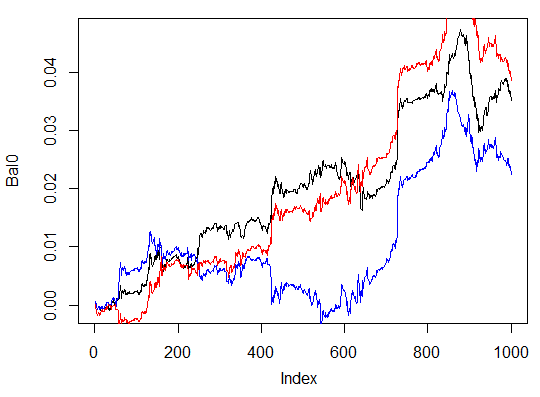
Fig. 30. Balance on the last 1000 bars by the signals of three neural networks with different numbers of hidden neurons
The results show that the third variant is the best out of the three with the maximum profit of 543 points. We only changed the number of hidden neurons and it led to a significant improvement. Searching of optimal parameters should be performed through evolutionary algorithms. This is up to the reader to explore.
It should be kept in mind that the author's algorithm has not been fully implemented in this package.
4. The Implementation (Indicator and Expert Advisor)
Now we are going to write a program for the indicator and Expert Advisor using a deep network for receiving trading signals.
There are two ways of such an implementation:
- The first one. Training of the neural network is performed in Rstudio manually. After obtaining acceptable results, save the network in the appropriate catalog. Then launch the EA and indicator on the chart. The EA will load the trained network. The indicator prepares a vector of new input data on each new bar and passes it to the EA. The EA presents network data, receives a signal and then acts on it. The EA is carrying on with its usual activities such as opening and closing orders, trailing etc The objective of the indicator is to prepare and pass on to the EA new input data on each new bar and, most importantly, present signals forecast by the network on a chart. Practice shows that visual control is the most efficient way of assessing a neural network.
- Second way. Launch the EA and the indicator on the chart. At the first launch, the indicator passes on to the EA a prepared large set of input and output data. The EA launches training, testing and selecting the best neural network. After that work goes on like in the first way.
We are going to write the link indicator-EA following the first algorithm. EA with a minimum of bows and frills.
Why is it so difficult? This way of implementation allows to connect several indicators placed on different symbols/timeframes to one EA and work with them consequently. For that, the EA has to go through a little modernization. We are going to talk about it later.
Below is the structure of interaction between the indicator and the EA:
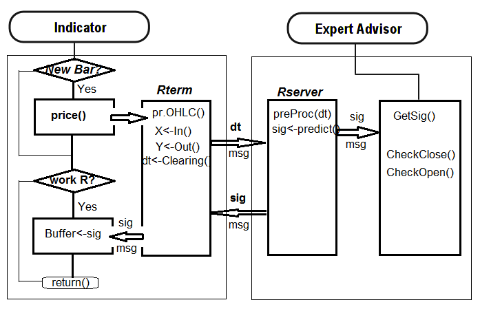
Fig. 31. Structure of interaction between the indicator and the EA
4.1. Training and Saving the Model
Using the indicator placed on the chart of our interest, obtain the necessary source data. For that, place the indicator on the chart, having set an input variable send=false, i.e. the visual representation is not supposed to get sent to the server. At the first launch on this symbol or timeframe, the indicator is to create the following directories /Symbol/TF/Test_Data/ in the data file of the terminal (/MQL4/Files).
Such an organization of directories gives an opportunity not to put experiment results together at preliminary training of models and not overwrite old data with new ones. Intermediary results will be stored in the /Symbol/TF/Test_Data/ directory and the model the EA is going to use for work will be located in /Symbol/TF/ (it will have to be placed there manually). The same result will be at the first launch on a new symbol or the EA's timeframe.
So, for EURUSD, М30, there are 4000 bars on 14.10.2014. We require the dt[] dataframe.
Balance classes:
> dt.b<-Balancing(dt)
> table(dt.b[ ,ncol(dt.b)])
   0    1
2288 2288
Now, with the previously written function Testing.1(), train the deep neural network with 500 and 300 epochs and assess the balance obtained on the last 500 bars by the signals forecast by the neural network.
> system.time(bal<-Testing.1(dt.b, dt, h = c(50, 50, 50), LR = 0.7, dec = 2, Ep=500, bar=500))
begin to train sae ......
training layer 1 autoencoder ...
####loss on step 10000 is : 0.000017
####loss on step 20000 is : 0.000015
####loss on step 30000 is : 0.000015
training layer 2 autoencoder ...
####loss on step 10000 is : 0.000044
####loss on step 20000 is : 0.000041
####loss on step 30000 is : 0.000039
training layer 3 autoencoder ...
####loss on step 10000 is : 0.000042
####loss on step 20000 is : 0.000042
####loss on step 30000 is : 0.000036
sae has been trained.
begin to train deep nn ......
####loss on step 10000 is : 0.089417
####loss on step 20000 is : 0.043276
####loss on step 30000 is : 0.069399
deep nn has been trained.
   user  system elapsed
 267.59    0.08  269.37
> plot(bal, t="l")
Save the neural network under a different name and train another one
> SAE1<-SAE
> system.time(bal<-Testing.1(dt.b, dt, h = c(50, 50, 50), LR = 0.7, dec = 2, Ep=300, bar=500))
begin to train sae ......
training layer 1 autoencoder ...
####loss on step 10000 is : 0.000020
####loss on step 20000 is : 0.000016
training layer 2 autoencoder ...
####loss on step 10000 is : 0.000050
####loss on step 20000 is : 0.000050
training layer 3 autoencoder ...
####loss on step 10000 is : 0.000051
####loss on step 20000 is : 0.000043
sae has been trained.
begin to train deep nn ......
####loss on step 10000 is : 0.083888
####loss on step 20000 is : 0.083941
deep nn has been trained.
   user  system elapsed
 155.32    0.02  156.25
> lines(bal, col=2)
Take a look at the balance charts (the last result highlighted in red).
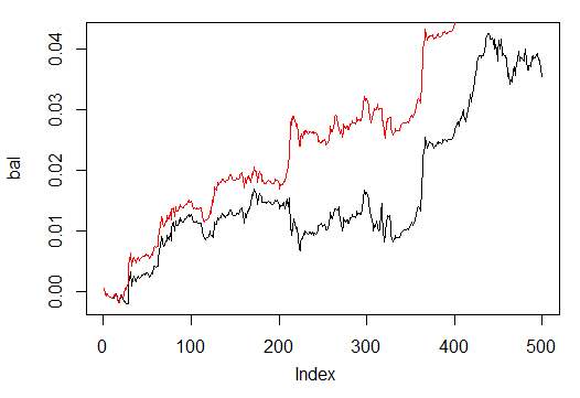
Fig. 32. Balance on the last 500 bars by the signals of neural networks trained in 500 and 300 epochs
As we can see, neural network trained in 300 epochs, showed a better result than the network trained in 500 epochs.
The training time of the latter is suitable for quick retraining during a trading session on this timeframe.
For further work on a real chart we need two objects: trained model "SAE" and normalization parameters "prepr" for input data. Save them in the relevant directory, in my case this is "D:/Alpari Limited MT4/MQL4/Files/EURUSD/M30/Test_2014-10-14". This is defined and operates as a working one, if you opened in Rstudio the "i_SAE_EURUSD_30.Rdata" working area saved by the indicator.
save(SAE, prepr, file="SAE.model")
In the "SAE.model" file, we saved the model itself and normalization parameters. Using the model without them does not make sense. You can experiment and save the models you like every day. They will be saved in the folders "/File/Symbol/TF/Test_Data". For the EA to use the model, put the "SAE.model" file to the folder "File/Symbol/TF/" manually. This folder can contain only one model and the EA will use it for work.
Having loaded the "SAE.model" file, the EA loads these objects to the working area for using in work. At this point the manual part of the work is finished, you can place the indicator-EA to the chart and test it in real time.
To assess the effectiveness of the EA's work, quantitative criteria are required. The Accuracy coefficient is not quite suitable for this purpose.
The average of the balance forecast ratio received by ZigZag and the balance ratio on the last bar to the number of bars. In our case this is the balance by ZigZag:
sig.zz<-ifelse(tail(dt[  , ncol(dt)], 500) == 0, 1, -1)
bal.zz<-cumsum(tail(price[  , 'CO'], 500) * sig.zz)
Kzz<-mean(bal.zz / bal)
> Kzz
[1] 0.9173312
This is a very high score but it is relative.
If we see what it looks like over time, we can see that for the first 50-100 bars this is an unstable index, though later it becomes nearly constant. Statistics are below:
> plot(bal/bal.zz, t="l")
> summary(bal/bal.zz)
    Min.  1st Qu.   Median     Mean  3rd Qu.     Max.
-15.2500   0.7341   0.7844   0.9173   0.8833  55.0000
Fig. 33. Ratio of the forecast balance to the balance obtained by ZigZag
The second one is more precise as it shows how many points of profit there are for one bar on a stretch N bars long.
For example, for the balance by neural network forecast on the stretch of 500 bars:
> Kb<-tail(bal,1)/length(bal)*10^Dig
> Kb
[1] 11.508
by ZigZag signals:
> Kbz<-tail(bal.zz,1)/length(bal)*10^Dig
> Kbz
[1] 13.784
When the lower limit of effectiveness on one of the parameters is defined, we know the time when we can retrain the neural network or optimize its parameters.
The EA will display the following parameters on the chart: OP – executed operation, Acc – Accuracy, K – is Kb defined earlier, Kmax – the same parameter as Kb but defined on the balance high and gives an idea of how much this parameter differs on the last bar from the maximal one.
4.2. Installation and Launching Order
In the attached archive SAE.zip you can find:
- The i_SAE.mq4 indicator, put to the ~/MQL4/Indicators/ folder
- The e_SAE.mq4 EA, put to the ~/MQL4/Experts/ folder
- The mt4Rb7.dll library, put to the ~/MQL4/Libraries/ folder.
- The mt4Rb7.mqh header file, put to the ~/MQL4/Include/ folder. The library and header file were developed and kindly provided by Bernd Kreuss. The name includes the index of the last change (b7). When there are a lot of versions with the same names, there are confusions that take a lot of time to rectify.
- Scripts on R: i_SAE.r (main indicator script), i_SAE_fun.r (functions of the indicator script), e_SAE.r (EA script), e_SAE_init.r (EA initialization script), SAE_SetDir.r (script of validation and creation of necessary directories). As scripts depend neither from the symbol, nor from a timefreame, they can be located in a separate directory. In my case this is "C:Rdata/SAE/". The "C:Rdata/" directory contains different scripts not attached to any certain project. If you put scripts in a folder different from mine, then make appropriate corrections in the indicator and EA that is correct the way to the scripts.
- SAE.model is a file with the "SAE" model and normalization parameters "prepr". The model was trained on EURUSD (M30), last date 14.10.14. The training process was described above.
Also do not forget the way to the directory where the R language was stored on your computer.
The following order is preferable to follow to start working. Place the EA on the chart. If you decide to place an EA on another symbol, a port, different from previously launched servers is to be specified. For instance, port 8886 (by default port 8888).
Note. This is an absolutely inefficient way. Every server has a size of 120-130 Mb. This is what things are today.
After normal EA initialization, the alert "No calculation results! Symbol" will appear. Then install the indicator with external parameter send = true and specified server port that the indicator is to connect to (see above). If everything works correctly, the real data "operation", Accuracy, K and Kmax will appear in the output string and trading will start.
Efficient control of the process can be best facilitated from the Windows Task Manager. If Rterm does not appear in the list after the EA or indicator was launched, then the R process was disrupted. The main reason of such disruptions is a syntax error in scripts, mismatch of the length of the receiving MQL vector and the vector extracted from Rterm.
Scripts can be debugged in Rstudio by launching scripts line by line from the beginning to the end.
Unfortunately I was unable to launch the EA in the tester, therefore it has to be tested on a demo account.
4.3. Ways and Methods of Improving Qualitative Characteristics
- Change the set of the indicators used at the input.
- Change the way of the input data normalization.
- Optimize parameters of the "supervisor" and indicators at the input.
- Change the coding of the input variable for the matrix with two columns. Calibrate the forecast signal.
- Optimize the network parameters (number of neurons in the hidden layers, number of layers, level of learning, number of epochs).
Conclusion
We have created, trained and tested deep network models with initialization of the neuron weights in the hidden layers from SAE. Networks retrain very quickly and it allows to retrain them without disrupting the trading process.
The results shown by neural networks are average in terms of metrics. The ideal result was not the initial goal.
Using such a model and permanent evaluation of the effectiveness coefficient, the model can be retrained and optimized without disrupting the trading process.
Attachment:
- SAE.zip - indicator, EA and accompanying files.
- R_intro.zip - literature on R and Rstudio in Rusian.
- DeepLearning.zip - literature of Deep Learning.
Translated from Russian by MetaQuotes Ltd.
Original article: https://www.mql5.com/ru/articles/1103
 Trader's Statistical Cookbook: Hypotheses
 Neural Networks Cheap and Cheerful - Link NeuroPro with MetaTrader 5
 Building an Interactive Application to Display RSS Feeds in MetaTrader 5
 Programming EA's Modes Using Object-Oriented Approach
- Free trading apps
- Over 8,000 signals for copying
- Economic news for exploring financial markets
You agree to website policy and terms of use
Using Rsi could be the wrong approach.
Maybe its a better one to let it trade directly, like as if it needs to learn to walk, or play chess or any other game.
pr.sae<-nn.predict(SAE, x.ts)
sig<-ifelse(pr.sae>mean(pr.sae), -1, 1)
sig.zz<-ifelse(y.ts == 0, 1,-1 )
bal<-cumsum(tail(price[ ,'CO'], bar) * sig)
bal.zz<-cumsum(tail(price[ ,'CO'], bar) * sig.zz)
sir, above code, when calc bal you havent move the sign backword like you did in the ariticle DEEP NEURAL NETDEEP NEURAL NETWORK WITH STACKED RBM.
sth do I miss?
Hi Fabio,
I'm sorry.
I do not write on MKL5.
Best regards
Vladimir
Hi Fabio,
What's not clear?
Hi Vladimir,
I don't have the vector of (o,h,l,c) in RStudio, How to download data in R and work with them in RStudio? when I run "head(price)" this massge shown:
> head(price)
Error in head(price) : object 'price' not found
> # The MT4 numbering bars from the most recent to oldest. The R on the contrary,
> # from the old to the new, new bar last, then use "rev" function to reverse this.
> price <- cbind(Open = rev(o), High = rev(h), Low = rev(l), Close = rev(c))
Error in rev(o) : object 'o' not found
Hi,
Thanks for sharing the information
On this:
save(SAE, prepr, file="SAE.model")How we can save the prepr?
I'm afraid the one I'm saving is not the same like the one in your model.
Could you please elaborate a little bit more.
Thanks.
Hi/
I am glad that you are interested in article.
Idebugcasesfall Rterma as follows:
- Comment out everything in the start () except that inspection workRterma
- Comment out in the init () all but runRterm()
- If Rterm is up and running, sinceInit()uncommentone operator and checked. Youspecifyat whathappens operator crash.
Thereafter easier to determine the cause crash.Usuallythere are two: the script syntax error orlack of necessarylibraries.
I again refer to Appendixto the article.
Ready to help you in the future if you tell whichfallsRterm.
Best regards
Did you manage to solve this, I got the same error too. Here is a snapshot. In my case the function RIsRunning(hR) is false in the get go. So, in the if statement it, crashes. Do we need this RIsRunning(hR) running? What does it do? Any way we could run it before hand by clicking the executable?
How did you solve this?