Matrix and Vector operations in MQL5

MetaQuotes | 26 September, 2022

Special data types — matrices and vectors — have been added to the MQL5 language to solve a large class of mathematical problems. The new types offer built-in methods for creating concise and understandable code that is close to mathematical notation. In this article, we provide a brief description of built-in methods from the Matrix and vector methods help section.

Every programming language offers array data types which store sets of numeric variables, including int, double and others. Array elements are accessed by index which enables array operations using loops. The most commonly used are one-dimensional and two-dimensional arrays:

int    a[50];       // One-dimensional array of 50 integers
double m[7][50];    // Two-dimensional array of 7 subarrays, each consisting of 50 integers
MyTime t[100];      // Array containing elements of MyTime type

The capabilities of arrays are usually enough for relatively simple tasks related to data storing and processing. But when it comes to complex mathematical problems, working with arrays becomes difficult in terms of both programming and code reading, due to the large number of nested loops. Even the simplest linear algebra operations require excessive coding and a good understanding of mathematics.

Modern data technologies such as machine learning, neural networks and 3D graphics, widely use linear algebra solutions associated with the concepts of vectors and matrices. To facilitate operations with such objects, MQL5 provides special data types: matrices and vectors. The new types eliminate a lot of routine programming operations and improve code quality.

Matrix and vector types

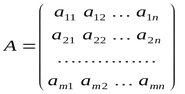
In short, a vector is a one-dimensional double-type array, and a matrix is a two-dimensional double-type array. Vectors can be vertical and horizontal; however, they are not separated in MQL5.

A matrix can be represented as an array of horizontal vectors, in which the first index is the row number, and the second index is the column number.

Row and column numbering starts from 0, similar to arrays.

In addition to 'matrix' and 'vector' types which contain double-type data, there are four more types for operations with the relevant data types:

matrixf — a matrix containing float elements
matrixc — a matrix containing complex elements
vectorf — a vector containing float elements
vectorc — a vector containing complex elements

At the time of this writing, work on the matrixc and vectorc types has not yet been completed, and thus it is not yet possible to use these types in built-in methods.

Template functions support notations like matrix<double>, matrix<float>, vector<double>, vector<float> instead of the corresponding types.

  vectorf       v_f1= {0, 1, 2, 3,};
  vector<float> v_f2=v_f1;
  Print("v_f2 = ", v_f2);

  /*
  v_f2 = [0,1,2,3]
  */

Creation and initialization

Matrix and vector methods are divided into nine categories according to their purpose. There are several ways to declare and initialize matrices and vectors.

The simplest creation method is declaration without size specification, that is, without memory allocation for the data. Here, we just write the data type and the variable name:

  matrix         matrix_a;   // double type matrix
  matrix<double> matrix_a1;  // another way to declare a double matrix, suitable for use in templates
  matrix<float>  matrix_a3;  // float type matrix
  vector         vector_a;   // double type vector
  vector<double> vector_a1;  // another notation to create a double vector
  vector<float>  vector_a3;  // float type vector

Then you can change the size of the created objects and fill them with the desired values. They can also be used in built-in matrix methods to obtain calculation results.

A matrix or a vector can be declared with the specified size, while allocating memory for the data but not initializing anything. Here, after the variable name, specify the size(s) in parentheses:

  matrix         matrix_a(128,128);           // the parameters can be either constants
  matrix<double> matrix_a1(InpRows,InpCols);  // or variables
  matrix<float>  matrix_a3(InpRows,1);        // analogue of a vertical vector
  vector         vector_a(256);
  vector<double> vector_a1(InpSize);
  vector<float>  vector_a3(InpSize+16);       // expression can be used as a parameter

The third way to create objects is to declare with initialization. In this case, matrix and vector sizes are determined by the initialization sequence indicated in curly braces:

  matrix         matrix_a={{0.1,0.2,0.3},{0.4,0.5,0.6}};
  matrix<double> matrix_a1=matrix_a;                      // the matrices must be of the same type
  matrix<float>  matrix_a3={{1,2},{3,4}};
  vector         vector_a={-5,-4,-3,-2,-1,0,1,2,3,4,5};
  vector<double> vector_a1={1,5,2.4,3.3};
  vector<float>  vector_a3=vector_a2;                     // the vectors must be of the same type

There are also static methods for creating matrices and vectors of the specified size, initialized in a certain way:

  matrix         matrix_a =matrix::Eye(4,5,1);
  matrix<double> matrix_a1=matrix::Full(3,4,M_PI);
  matrixf        matrix_a2=matrixf::Identity(5,5);
  matrixf<float> matrix_a3=matrixf::Ones(5,5);
  matrix         matrix_a4=matrix::Tri(4,5,-1);
  vector         vector_a =vector::Ones(256);
  vectorf        vector_a1=vector<float>::Zeros(16);
  vector<float>  vector_a2=vectorf::Full(128,float_value);

In addition, there are non-static methods for initializing a matrix or a vector with the given values — Init and Fill:

  matrix m(2, 2);
  m.Fill(10);
  Print("matrix m \n", m);
  /*
  matrix m
  [[10,10]
  [10,10]]
  */
  m.Init(4, 6);
  Print("matrix m \n", m);
  /*
  matrix m
  [[10,10,10,10,0.0078125,32.00000762939453]
  [0,0,0,0,0,0]
  [0,0,0,0,0,0]
  [0,0,0,0,0,0]]
  */

In this example, we used the Init method to change the sizes of an already initialized matrix, due to which all new elements were filled with random values.

An important advantage of the Init method is the ability to specify an initializing function in parameters to fill matrix/vector elements according to this rule. For example:

void OnStart()
 {
//---
  matrix init(3, 6, MatrixSetValues);  
  Print("init = \n", init);
  /*
  Execution result
  init = 
  [[1,2,4,8,16,32]
   [64,128,256,512,1024,2048]
   [4096,8192,16384,32768,65536,131072]]
  */   
 }
//+------------------------------------------------------------------+
//| Fills the matrix with powers of a number                         |
//+------------------------------------------------------------------+
void MatrixSetValues(matrix& m, double initial=1)
 {
  double value=initial;
  for(ulong r=0; r<m.Rows(); r++)
   {
    for(ulong c=0; c<m.Cols(); c++)
     {
      m[r][c]=value;
      value*=2;
     }
   }
 }

Copying matrices and arrays

Matrices and vectors can be copied using the Copy method. But a simpler and a more familiar way to copy these data types is to use the assignment operator "=". Also, you can use the Assign method for copying.

//--- copying matrices
  matrix a= {{2, 2}, {3, 3}, {4, 4}};
  matrix b=a+2;
  matrix c;
  Print("matrix a \n", a);
  Print("matrix b \n", b);
  c.Assign(b);
  Print("matrix c \n", c);
  /*
   matrix a
   [[2,2]
    [3,3]
    [4,4]]
   matrix b
   [[4,4]
    [5,5]
    [6,6]]
   matrix c
   [[4,4]
    [5,5]
    [6,6]]
  */

The difference of Assign from Copy is that it can be used for both matrices and arrays. The example below shows copying of the integer array int_arr into a double matrix. The resulting matrix automatically adjusts according to the size of the copied array.

//--- copying an array to a matrix
  matrix double_matrix=matrix::Full(2,10,3.14);
  Print("double_matrix before Assign() \n", double_matrix);
  int int_arr[5][5]= {{1, 2}, {3, 4}, {5, 6}};
  Print("int_arr: ");
  ArrayPrint(int_arr);
  double_matrix.Assign(int_arr);
  Print("double_matrix after Assign(int_arr) \n", double_matrix);  
  /*
   double_matrix before Assign() 
   [[3.14,3.14,3.14,3.14,3.14,3.14,3.14,3.14,3.14,3.14]
    [3.14,3.14,3.14,3.14,3.14,3.14,3.14,3.14,3.14,3.14]]
    
   int_arr: 
       [,0][,1][,2][,3][,4]
   [0,]   1   2   0   0   0
   [1,]   3   4   0   0   0
   [2,]   5   6   0   0   0
   [3,]   0   0   0   0   0
   [4,]   0   0   0   0   0
   
   double_matrix after Assign(int_arr) 
   [[1,2,0,0,0]
    [3,4,0,0,0]
    [5,6,0,0,0]
    [0,0,0,0,0]
    [0,0,0,0,0]]
  */
 }

The Assign method enables seamless transition from arrays to matrices, with the automated size and type casting.

Copying timeseries to matrices or vectors

Price chart analysis implies operations with MqlRates structure arrays. MQL5 provides a new method for working with such price data structures.

The CopyRates method copies historical series of the MqlRates structure directly into a matrix or vector. Thus, you can avoid the need to get the required timeseries into the relevant arrays using functions from the Timeseries and indicator access section. Also, there is no need to transfer them to a matrix or vector. With the CopyRates method, you can receive quotes into a matrix or vector in just one call. Let's consider an example of how to calculate a correlation matrix for a list of symbols: let's calculate these values using two different methods and compare the results.

input int             InBars=100;
input ENUM_TIMEFRAMES InTF=PERIOD_H1;
//+------------------------------------------------------------------+
//| Script program start function                                    |
//+------------------------------------------------------------------+
void OnStart()
 {
//--- list of symbols for calculation
  string symbols[]= {"EURUSD", "GBPUSD", "USDJPY", "USDCAD", "USDCHF"};
  int size=ArraySize(symbols);
//--- matrix and vector to receive Close prices
  matrix rates(InBars, size);
  vector close;
  for(int i=0; i<size; i++)
   {
    //--- get Close prices to a vector
    if(close.CopyRates(symbols[i], InTF, COPY_RATES_CLOSE, 1, InBars))
     {
      //--- insert the vector to the timeseries matrix
      rates.Col(close, i);
      PrintFormat("%d. %s: %d Close prices were added to matrix", i+1, symbols[i], close.Size());
      //--- output the first 20 vector values for debugging
      int  digits=(int)SymbolInfoInteger(symbols[i], SYMBOL_DIGITS);
      Print(VectorToString(close, 20, digits));
     }
    else
     {
      Print("vector.CopyRates(%d,COPY_RATES_CLOSE) failed. Error ", symbols[i], GetLastError());
      return;
     }
   }
  /*
  1. EURUSD: 100 Close prices were added to the matrix
  0.99561 0.99550 0.99674 0.99855 0.99695 0.99555 0.99732 1.00305 1.00121   1.069 0.99936   1.027 1.00130 1.00129 1.00123 1.00201 1.00222 1.00111   1.079   1.030  ...
  2. GBPUSD: 100 Close prices were added to the matrix
  1.13733 1.13708 1.13777 1.14045 1.13985 1.13783 1.13945 1.14315 1.14172 1.13974 1.13868 1.14116 1.14239 1.14230 1.14160 1.14281 1.14338 1.14242 1.14147 1.14069  ...
  3. USDJPY: 100 Close prices were added to the matrix
  143.451 143.356 143.310 143.202 143.079 143.294 143.146 142.963 143.039 143.032 143.039 142.957 142.904 142.956 142.920 142.837 142.756 142.928 143.130 143.069  ...
  4. USDCAD: 100 Close prices were added to the matrix
  1.32840 1.32877 1.32838 1.32660 1.32780 1.33068 1.33001 1.32798 1.32730 1.32782 1.32951 1.32868 1.32716 1.32663 1.32629 1.32614 1.32586 1.32578 1.32650 1.32789  ...
  5. USDCHF: 100 Close prices were added to the matrix
  0.96395 0.96440 0.96315 0.96161 0.96197 0.96337 0.96358 0.96228 0.96474 0.96529 0.96529 0.96502 0.96463 0.96429 0.96378 0.96377 0.96314 0.96428 0.96483 0.96509  ...
  */
//--- prepare a matrix of correlations between symbols
  matrix corr_from_vector=matrix::Zeros(size, size);
  Print("Compute pairwise correlation coefficients");
  for(int i=0; i<size; i++)
   {
    for(int k=i; k<size; k++)
     {
      vector v1=rates.Col(i);
      vector v2=rates.Col(k);
      double coeff = v1.CorrCoef(v2);
      PrintFormat("corr(%s,%s) = %.3f", symbols[i], symbols[k], coeff);
      corr_from_vector[i][k]=coeff;
     }
   }
  Print("Correlation matrix on vectors: \n", corr_from_vector);
  /*
  Calculate pairwise correlation coefficients
  corr(EURUSD,EURUSD) = 1.000
  corr(EURUSD,GBPUSD) = 0.974
  corr(EURUSD,USDJPY) = -0.713
  corr(EURUSD,USDCAD) = -0.950
  corr(EURUSD,USDCHF) = -0.397
  corr(GBPUSD,GBPUSD) = 1.000
  corr(GBPUSD,USDJPY) = -0.744
  corr(GBPUSD,USDCAD) = -0.953
  corr(GBPUSD,USDCHF) = -0.362
  corr(USDJPY,USDJPY) = 1.000
  corr(USDJPY,USDCAD) = 0.736
  corr(USDJPY,USDCHF) = 0.083
  corr(USDCAD,USDCAD) = 1.000
  corr(USDCAD,USDCHF) = 0.425
  corr(USDCHF,USDCHF) = 1.000

  Correlation matrix on vectors:
  [[1,0.9736363791537366,-0.7126365191640618,-0.9503129578410202,-0.3968181226230434]
   [0,1,-0.7440448047501974,-0.9525190338388175,-0.3617774666815978]
   [0,0,1,0.7360546499847362,0.08314381248168941]
   [0,0,0,0.9999999999999999,0.4247042496841555]
   [0,0,0,0,1]]
  */
//--- now let's see how a correlation matrix can be calculated in one line
  matrix corr_from_matrix=rates.CorrCoef(false);   // false means that the vectors are in the matrix columns
  Print("Correlation matrix rates.CorrCoef(false): \n", corr_from_matrix.TriU());
//--- compare the resulting matrices to find discrepancies
  Print("How many discrepancy errors between result matrices?");
  ulong errors=corr_from_vector.Compare(corr_from_matrix.TriU(), (float)1e-12);
  Print("corr_from_vector.Compare(corr_from_matrix,1e-12)=", errors);
  /*
  Correlation matrix rates.CorrCoef(false):
  [[1,0.9736363791537366,-0.7126365191640618,-0.9503129578410202,-0.3968181226230434]
   [0,1,-0.7440448047501974,-0.9525190338388175,-0.3617774666815978]
   [0,0,1,0.7360546499847362,0.08314381248168941]
   [0,0,0,1,0.4247042496841555]
   [0,0,0,0,1]]

  How many discrepancy errors between result matrices?
  corr_from_vector.Compare(corr_from_matrix,1e-12)=0
  */
//--- create a nice output of the correlation matrix
  Print("Output the correlation matrix with headers");
  string header="        ";  // header
  for(int i=0; i<size; i++)
    header+="  "+symbols[i];
  Print(header);
//--- now rows
  for(int i=0; i<size; i++)
   {
    string line=symbols[i]+"  ";
    line+=VectorToString(corr_from_vector.Row(i), size, 3, 8);
    Print(line);
   }
  /*
  Output the correlation matrix with headers
            EURUSD  GBPUSD  USDJPY  USDCAD  USDCHF
  EURUSD       1.0   0.974  -0.713  -0.950  -0.397
  GBPUSD       0.0     1.0  -0.744  -0.953  -0.362
  USDJPY       0.0     0.0     1.0   0.736   0.083
  USDCAD       0.0     0.0     0.0     1.0   0.425
  USDCHF       0.0     0.0     0.0     0.0     1.0
  */
 }
//+------------------------------------------------------------------+
//| Returns a string with vector values                              |
//+------------------------------------------------------------------+
string VectorToString(const vector &v, int length=20, int digits=5, int width=8)
 {
  ulong size=(ulong)MathMin(20, v.Size());
//--- compose a string
  string line="";
  for(ulong i=0; i<size; i++)
   {
    string value=DoubleToString(v[i], digits);
    StringReplace(value, ".000", ".0");
    line+=Indent(width-StringLen(value))+value;
   }
  //--- add a tail if the vector length exceeds the specified size
  if(v.Size()>size)
    line+="  ...";
//---
  return(line);
 }
//+------------------------------------------------------------------+
//|  Returns a string with the specified number of spaces            |
//+------------------------------------------------------------------+
string Indent(int number)
 {
  string indent="";
  for(int i=0; i<number; i++)
    indent+=" ";
  return(indent);
 }

The example shows how to:

Get Close prices using CopyRates
Insert a vector into a matrix using the Col method
Calculate the correlation coefficient between two vectors using CorrCoef
Calculate the correlation matrix over a matrix with value vectors using CorrCoef
Return an upper triangular matrix using the TriU method
Compare two matrices and find discrepancies using Compare

Matrix and vector operations

Element-wise mathematical operations of addition, subtraction, multiplication and division can be performed on matrices and vectors. Both objects in such operations must be of the same type and must have the same sizes. Each element of the matrix or vector operates on the corresponding element of the second matrix or vector.

You can also use a scalar of the appropriate type (double, float or complex) as the second term (multiplier, subtrahend or divisor). In this case, each member of the matrix or vector will operate on the specified scalar.

  matrix matrix_a={{0.1,0.2,0.3},{0.4,0.5,0.6}};
  matrix matrix_b={{1,2,3},{4,5,6}};
  matrix matrix_c1=matrix_a+matrix_b;
  matrix matrix_c2=matrix_b-matrix_a;
  matrix matrix_c3=matrix_a*matrix_b;   // Hadamard product
  matrix matrix_c4=matrix_b/matrix_a;
  matrix_c1=matrix_a+1;
  matrix_c2=matrix_b-double_value;
  matrix_c3=matrix_a*M_PI;
  matrix_c4=matrix_b/0.1;
//--- operations in place are possible
  matrix_a+=matrix_b;
  matrix_a/=2;

In addition, matrices and vectors can be passed as a second parameter to most mathematical functions, including MathAbs, MathArccos, MathArcsin, MathArctan, MathCeil, MathCos, MathExp, MathFloor, MathLog, MathLog10, MathMod, MathPow, MathRound, MathSin, MathSqrt, MathTan, MathExpm1, MathLog1p, MathArccosh, MathArcsinh, MathArctanh, MathCosh, MathSinh, MathTanh. Such operations imply element-wise handling of matrices or vectors. Example:

//---
  matrix a= {{1, 4}, {9, 16}};
  Print("matrix a=\n",a);
  a=MathSqrt(a);
  Print("MatrSqrt(a)=\n",a);
  /*
   matrix a=
   [[1,4]
    [9,16]]
   MatrSqrt(a)=
   [[1,2]
    [3,4]]
  */

For MathMod and MathPow, the second element can be either a scalar or a matrix/vector of the appropriate size.

   matrix<T> mat1(128,128);
   matrix<T> mat3(mat1.Rows(),mat1.Cols());
   ulong     n,size=mat1.Rows()*mat1.Cols();
...
   mat2=MathPow(mat1,(T)1.9);
   for(n=0; n<size; n++)
     {
      T res=MathPow(mat1.Flat(n),(T)1.9);
      if(res!=mat2.Flat(n))
         errors++;
     }

   mat2=MathPow(mat1,mat3);
   for(n=0; n<size; n++)
     {
      T res=MathPow(mat1.Flat(n),mat3.Flat(n));
      if(res!=mat2.Flat(n))
         errors++;
     }
...
   vector<T> vec1(16384);
   vector<T> vec3(vec1.Size());
   ulong     n,size=vec1.Size();
...
   vec2=MathPow(vec1,(T)1.9);
   for(n=0; n<size; n++)
     {
      T res=MathPow(vec1[n],(T)1.9);
      if(res!=vec2[n])
         errors++;
     }
   vec2=MathPow(vec1,vec3);
   for(n=0; n<size; n++)
     {
      T res=MathPow(vec1[n],vec3[n]);
      if(res!=vec2[n])
         errors++;
     }

Manipulations

MQL5 supports the following basic manipulations on matrices and vectors, which do not require any calculations:

Transposition
Extracting rows, columns and diagonals
Resizing and reshaping matrices
Swapping the specified rows and columns
Copying to a new object
Comparing two objects
Splitting a matrix into multiple submatrices
Sorting

The following example shows matrix transposition using the Transpose method:

  matrix a= {{0, 1, 2}, {3, 4, 5}};
  Print("matrix a \n", a);
  Print("a.Transpose() \n", a.Transpose());
  /*
  matrix a
  [[0,1,2]
   [3,4,5]]
  a.Transpose()
  [[0,3]
   [1,4]
   [2,5]]
  */

Below are examples showing how to set and extract a diagonal using the Diag method:

   vector v1={1,2,3};
   matrix m1;
   m1.Diag(v1);
   Print("m1\n",m1);
  /* 
  m1
  [[1,0,0]
  [0,2,0]
  [0,0,3]]
  m2
  */

   matrix m2;
   m2.Diag(v1,-1);
   Print("m2\n",m2);
  /*
  m2
  [[0,0,0]
  [1,0,0]
  [0,2,0]
  [0,0,3]]
  */

   matrix m3;
   m3.Diag(v1,1);
   Print("m3\n",m3);
  /*
  m3
  [[0,1,0,0]
  [0,0,2,0]
  [0,0,0,3]]
  */

   matrix m4=matrix::Full(4,5,9);
   m4.Diag(v1,1);
   Print("m4\n",m4);
   
   Print("diag -1 - ",m4.Diag(-1));
   Print("diag 0 - ",m4.Diag());
   Print("diag 1 - ",m4.Diag(1)); 
  /*
  m4
  [[9,1,9,9,9]
  [9,9,2,9,9]
  [9,9,9,3,9]
  [9,9,9,9,9]]
  diag -1 - [9,9,9]
  diag 0 - [9,9,9,9]
  diag 1 - [1,2,3,9]
  */

Changing a matrix size using the Reshape method:

   matrix matrix_a={{1,2,3},{4,5,6},{7,8,9},{10,11,12}};
   Print("matrix_a\n",matrix_a);
  /*
  matrix_a
  [[1,2,3]
   [4,5,6]
   [7,8,9]
   [10,11,12]]

  */

   matrix_a.Reshape(2,6);
   Print("Reshape(2,6)\n",matrix_a);
  /*
  Reshape(2,6)
  [[1,2,3,4,5,6]
   [7,8,9,10,11,12]]
  */

   matrix_a.Reshape(3,5);
   Print("Reshape(3,5)\n",matrix_a);
  /*
  Reshape(3,5)
  [[1,2,3,4,5]
   [6,7,8,9,10]
   [11,12,0,3,0]]
  */

   matrix_a.Reshape(2,4);
   Print("Reshape(2,4)\n",matrix_a);
  /*
  Reshape(2,4)
  [[1,2,3,4]
   [5,6,7,8]]
  */

Examples of a vertical split of a matrix using the Vsplit method:

   matrix matrix_a={{ 1, 2, 3, 4, 5, 6},
                    { 7, 8, 9,10,11,12},
                    {13,14,15,16,17,18}};
   matrix splitted[];
   ulong  parts[]={2,3};
 
   matrix_a.Vsplit(2,splitted);
   for(uint i=0; i<splitted.Size(); i++)
      Print("splitted ",i,"\n",splitted[i]);
  /*
     splitted 0
     [[1,2,3]
      [7,8,9]
      [13,14,15]]
     splitted 1
     [[4,5,6]
      [10,11,12]
      [16,17,18]]
  */
 
   matrix_a.Vsplit(3,splitted);
   for(uint i=0; i<splitted.Size(); i++)
      Print("splitted ",i,"\n",splitted[i]);
  /* 
     splitted 0
     [[1,2]
      [7,8]
      [13,14]]
     splitted 1
     [[3,4]
      [9,10]
      [15,16]]
     splitted 2
     [[5,6]
      [11,12]
      [17,18]]
*/
 
   matrix_a.Vsplit(parts,splitted);
   for(uint i=0; i<splitted.Size(); i++)
      Print("splitted ",i,"\n",splitted[i]);
  /* 
     splitted 0
     [[1,2]
      [7,8]
      [13,14]]
     splitted 1
     [[3,4,5]
      [9,10,11]
      [15,16,17]]
     splitted 2
     [[6]
      [12]
      [18]]
  */

The Col and Row methods allow getting the relevant matrix elements as well as inserting elements into unallocated matrices, i.e. matrices without the specified size. Here is an example:

   vector v1={1,2,3};
   matrix m1;
   m1.Col(v1,1);
   Print("m1\n",m1);
  /*
   m1
   [[0,1]
    [0,2]
    [0,3]]
  */

   matrix m2=matrix::Full(4,5,8);
   m2.Col(v1,2);
   Print("m2\n",m2);
  /*
   m2
   [[8,8,1,8,8]
    [8,8,2,8,8]

    [8,8,3,8,8]
    [8,8,8,8,8]]   
  */

   Print("col 1 - ",m2.Col(1));
  /*
   col 1 - [8,8,8,8]
  */

   Print("col 2 - ",m2.Col(2));
  /*
   col 1 - [8,8,8,8]  col 2 - [1,2,3,8]
  */

Products

Matrix multiplication is one of the basic algorithms which is widely used in numerical methods. Many implementations of forward and back-propagation algorithms in neural network convolutional layers are based on this operation. Often, 90-95% of all time spent on machine learning is taken by this operation. All product methods are provided under the Products of matrices and vectors section of the language reference.

The following example shows the multiplication of two matrices using the MatMul method:

   matrix a={{1, 0, 0},
             {0, 1, 0}};
   matrix b={{4, 1},
             {2, 2},
             {1, 3}};
   matrix c1=a.MatMul(b);
   matrix c2=b.MatMul(a);
   Print("c1 = \n", c1);
   Print("c2 = \n", c2);
/*
   c1 = 
   [[4,1]
    [2,2]]
   c2 = 
   [[4,1,0]
    [2,2,0]
    [1,3,0]]
*/

An example of the Kronecker product of two matrices or a matrix and a vector, using the Kron method.

   matrix a={{1,2,3},{4,5,6}};
   matrix b=matrix::Identity(2,2);
   vector v={1,2};
 
   Print(a.Kron(b));
   Print(a.Kron(v));
 
  /*
   [[1,0,2,0,3,0]
    [0,1,0,2,0,3]
    [4,0,5,0,6,0]
    [0,4,0,5,0,6]]
 
   [[1,2,2,4,3,6]
    [4,8,5,10,6,12]]
  */

More examples from the article Matrices and Vectors in MQL5:

//--- initialize matrices
   matrix m35, m52;
   m35.Init(3,5,Arange);
   m52.Init(5,2,Arange);
//---
   Print("1. Product of horizontal vector v[3] and matrix m[3,5]");
   vector v3 = {1,2,3};
   Print("On the left v3 = ",v3);
   Print("On the right m35 = \n",m35);
   Print("v3.MatMul(m35) = horizontal vector v[5] \n",v3.MatMul(m35));
   /*
   1. Product of horizontal vector v[3] and matrix m[3,5]
   On the left v3 = [1,2,3]
   On the right m35 =
   [[0,1,2,3,4]
    [5,6,7,8,9]
    [10,11,12,13,14]]
   v3.MatMul(m35) = horizontal vector v[5]
   [40,46,52,58,64]
   */

//--- show that this is really a horizontal vector
   Print("\n2. Product of matrix m[1,3] and matrix m[3,5]");
   matrix m13;
   m13.Init(1,3,Arange,1);
   Print("On the left m13 = \n",m13);
   Print("On the right m35 = \n",m35);
   Print("m13.MatMul(m35) = matrix m[1,5] \n",m13.MatMul(m35));
   /*
   2. Product of matrix m[1,3] and matrix m[3,5]
   On the left m13 =
   [[1,2,3]]
   On the right m35 =
   [[0,1,2,3,4]
    [5,6,7,8,9]
    [10,11,12,13,14]]
   m13.MatMul(m35) = matrix m[1,5]
   [[40,46,52,58,64]]
   */

   Print("\n3. Product of matrix m[3,5] and vertical vector v[5]");
   vector v5 = {1,2,3,4,5};
   Print("On the left m35 = \n",m35);
   Print("On the right v5 = ",v5);
   Print("m35.MatMul(v5) = vertical vector v[3] \n",m35.MatMul(v5));
   /*
   3. Product of matrix m[3,5] and vertical vector v[5]
   On the left m35 =
   [[0,1,2,3,4]
    [5,6,7,8,9]
    [10,11,12,13,14]]
   On the right v5 = [1,2,3,4,5]
   m35.MatMul(v5) = vertical vector v[3]
   [40,115,190]
   */

//--- show that this is really a vertical vector
   Print("\n4. Product of matrix m[3,5] and matrix m[5,1]");
   matrix m51;
   m51.Init(5,1,Arange,1);
   Print("On the left m35 = \n",m35);
   Print("On the right m51 = \n",m51);
   Print("m35.MatMul(m51) = matrix v[3] \n",m35.MatMul(m51));
   /*
   4. Product of matrix m[3,5] and matrix m[5,1]
   On the left m35 =
   [[0,1,2,3,4]
    [5,6,7,8,9]
    [10,11,12,13,14]]
   On the right m51 =
   [[1]
    [2]
    [3]
    [4]
    [5]]
   m35.MatMul(m51) = matrix v[3]
   [[40]
    [115]
    [190]]
   */

   Print("\n5. Product of matrix m[3,5] and matrix m[5,2]");
   Print("On the left m35 = \n",m35);
   Print("On the right m52 = \n",m52);
   Print("m35.MatMul(m52) = matrix m[3,2] \n",m35.MatMul(m52));
   /*
   5. Product of matrix m[3,5] and matrix m[5,2]
   On the left m35 =
   [[0,1,2,3,4]
    [5,6,7,8,9]
    [10,11,12,13,14]]
   On the right m52 =
   [[0,1]
    [2,3]
    [4,5]
    [6,7]
    [8,9]]
   m35.MatMul(m52) = matrix m[3,2]
   [[60,70]
    [160,195]
    [260,320]]
   */

   Print("\n6. Product of horizontal vector v[5] and matrix m[5,2]");
   Print("On the left v5 = \n",v5);
   Print("On the right m52 = \n",m52);
   Print("v5.MatMul(m52) = horizontal vector v[2] \n",v5.MatMul(m52));
   /*
   6. The product of horizontal vector v[5] and matrix m[5,2]
   On the left v5 =
   [1,2,3,4,5]
   On the right m52 =
   [[0,1]
    [2,3]
    [4,5]
    [6,7]
    [8,9]]
   v5.MatMul(m52) = horizontal vector v[2]
   [80,95]
   */

   Print("\n7. Outer() product of horizontal vector v[5] and vertical vector v[3]");
   Print("On the left v5 = \n",v5);
   Print("On the right v3 = \n",v3);
   Print("v5.Outer(v3) = matrix m[5,3] \n",v5.Outer(v3));
   /*
   7. Outer() product of horizontal vector v[5] and vertical vector v[3]
   On the left v5 =
   [1,2,3,4,5]
   On the right v3 =
   [1,2,3]
   v5.Outer(v3) = matrix m[5,3]
   [[1,2,3]
    [2,4,6]
    [3,6,9]
    [4,8,12]
    [5,10,15]]
   */

Transformations

Matrix transformations are often used in data operations. However, many complex matrix operations cannot be solved efficiently or stably due to the limited accuracy of computers.

Matrix transformations (or decompositions) are methods which reduce a matrix into its component parts, which makes it easier to calculate more complex matrix operations. Matrix decomposition methods, also referred to as matrix factorization methods, are the backbone of linear algebra in computers, even for basic operations such as linear equation solving systems, calculating the inverse, and calculating the determinant of a matrix.

Machine learning widely uses Singular Value Decomposition (SVD), which enables the representation of the original matrix as the product of three other matrices. SVD is used to solve a variety of problems, from least squares approximation to compression and image recognition.

An example of a Singular Value Decomposition by the SVD method:

  matrix a= {{0, 1, 2, 3, 4, 5, 6, 7, 8}};
  a=a-4;
  Print("matrix a \n", a);
  a.Reshape(3, 3);
  matrix b=a;
  Print("matrix b \n", b);
//--- execute SVD decomposition
  matrix U, V;
  vector singular_values;
  b.SVD(U, V, singular_values);
  Print("U \n", U);
  Print("V \n", V);
  Print("singular_values = ", singular_values);
 
// check block
//--- U * singular diagonal * V = A
  matrix matrix_s;
  matrix_s.Diag(singular_values);
  Print("matrix_s \n", matrix_s);
  matrix matrix_vt=V.Transpose();
  Print("matrix_vt \n", matrix_vt);
  matrix matrix_usvt=(U.MatMul(matrix_s)).MatMul(matrix_vt);
  Print("matrix_usvt \n", matrix_usvt);
 
  ulong errors=(int)b.Compare(matrix_usvt, 1e-9);
  double res=(errors==0);
  Print("errors=", errors);
 
//---- another check
  matrix U_Ut=U.MatMul(U.Transpose());
  Print("U_Ut \n", U_Ut);
  Print("Ut_U \n", (U.Transpose()).MatMul(U));
 
  matrix vt_V=matrix_vt.MatMul(V);
  Print("vt_V \n", vt_V);
  Print("V_vt \n", V.MatMul(matrix_vt)); 
  /*
  matrix a
  [[-4,-3,-2,-1,0,1,2,3,4]]
  matrix b
  [[-4,-3,-2]
   [-1,0,1]
   [2,3,4]]
  U
  [[-0.7071067811865474,0.5773502691896254,0.408248290463863]
   [-6.827109697437648e-17,0.5773502691896253,-0.8164965809277256]
   [0.7071067811865472,0.5773502691896255,0.4082482904638627]]
  V
  [[0.5773502691896258,-0.7071067811865474,-0.408248290463863]
   [0.5773502691896258,1.779939029415334e-16,0.8164965809277258]
   [0.5773502691896256,0.7071067811865474,-0.408248290463863]]
  singular_values = [7.348469228349533,2.449489742783175,3.277709923350408e-17]
 
  matrix_s
  [[7.348469228349533,0,0]
   [0,2.449489742783175,0]
   [0,0,3.277709923350408e-17]]
  matrix_vt
  [[0.5773502691896258,0.5773502691896258,0.5773502691896256]
   [-0.7071067811865474,1.779939029415334e-16,0.7071067811865474]
   [-0.408248290463863,0.8164965809277258,-0.408248290463863]]
  matrix_usvt
  [[-3.999999999999997,-2.999999999999999,-2]
   [-0.9999999999999981,-5.977974170712231e-17,0.9999999999999974]
   [2,2.999999999999999,3.999999999999996]]
  errors=0
 
  U_Ut
  [[0.9999999999999993,-1.665334536937735e-16,-1.665334536937735e-16]
   [-1.665334536937735e-16,0.9999999999999987,-5.551115123125783e-17]
   [-1.665334536937735e-16,-5.551115123125783e-17,0.999999999999999]]
  Ut_U
  [[0.9999999999999993,-5.551115123125783e-17,-1.110223024625157e-16]
   [-5.551115123125783e-17,0.9999999999999987,2.498001805406602e-16]
   [-1.110223024625157e-16,2.498001805406602e-16,0.999999999999999]]
  vt_V
  [[1,-5.551115123125783e-17,0]
   [-5.551115123125783e-17,0.9999999999999996,1.110223024625157e-16]
   [0,1.110223024625157e-16,0.9999999999999996]]
  V_vt
  [[0.9999999999999999,1.110223024625157e-16,1.942890293094024e-16]
   [1.110223024625157e-16,0.9999999999999998,1.665334536937735e-16]
   [1.942890293094024e-16,1.665334536937735e-16,0.9999999999999996]
  */
 }

Another commonly used transformation is the Cholesky decomposition, which can be used to solve a system of linear equations Ax=b if the matrix A is symmetric and positive definite.

In MQL5, the Cholesky decomposition is executed by the Cholesky method:

  matrix matrix_a= {{5.7998084, -2.1825367}, {-2.1825367, 9.85910595}};
  matrix matrix_l;
  Print("matrix_a\n", matrix_a);
 
  matrix_a.Cholesky(matrix_l);
  Print("matrix_l\n", matrix_l);
  Print("check\n", matrix_l.MatMul(matrix_l.Transpose()));  
  /*
  matrix_a
  [[5.7998084,-2.1825367]
   [-2.1825367,9.85910595]]
  matrix_l
  [[2.408279136645086,0]
   [-0.9062640068544704,3.006291985133859]]
  check
  [[5.7998084,-2.1825367]
   [-2.1825367,9.85910595]]
  */

The below table shows the list of available methods:

Function	Action
Cholesky	Computes the Cholesky decomposition
Eig	Computes the eigenvalues and right eigenvectors of a square matrix
EigVals	Computes the eigenvalues of a general matrix
LU	LU factorization of a matrix as the product of a lower triangular matrix and an upper triangular matrix
LUP	LUP factorization with partial pivoting, which refers to LU decomposition with row permutations only: PA=LU
QR	Compute the qr factorization of a matrix
SVD	Singular Value Decomposition

Obtaining statistics

Methods from the Statistics section are used for computing descriptive statistics of matrices and vectors. Use them to find:

Maximum and minimum values, along with their indices in a matrix/vector
The sum and product of elements, as well as the cumulative sum and product
Median, mean, arithmetic mean and weighted arithmetic mean of matrix/vector values
Standard deviation and element variance
Percentiles and quantiles
Regression metric as the deviation error from the regression line constructed on the specified data array

An example of calculating the standard deviation by the Std method:

   matrixf matrix_a={{10,3,2},{1,8,12},{6,5,4},{7,11,9}};
   Print("matrix_a\n",matrix_a);
 
   vectorf cols_std=matrix_a.Std(0);
   vectorf rows_std=matrix_a.Std(1);
   float matrix_std=matrix_a.Std();
 
   Print("cols_std ",cols_std);
   Print("rows_std ",rows_std);
   Print("std value  ",matrix_std);
   /*
   matrix_a
   [[10,3,2]
    [1,8,12]
    [6,5,4]
    [7,11,9]]
   cols_std [3.2403703,3.0310888,3.9607449]
   rows_std [3.5590262,4.5460606,0.81649661,1.6329932]
   std value  3.452052593231201
   */

Calculating quantiles by the Quantile method:

   matrixf matrix_a={{1,2,3},{4,5,6},{7,8,9},{10,11,12}};
   Print("matrix_a\n",matrix_a);
 
   vectorf cols_percentile=matrix_a.Percentile(50,0);
   vectorf rows_percentile=matrix_a.Percentile(50,1);
   float matrix_percentile=matrix_a.Percentile(50);
 
   Print("cols_percentile ",cols_percentile);
   Print("rows_percentile ",rows_percentile);
   Print("percentile value  ",matrix_percentile);
   /*
   matrix_a
   [[1,2,3]
    [4,5,6]
    [7,8,9]
    [10,11,12]]
   cols_percentile [5.5,6.5,7.5]
   rows_percentile [2,5,8,11]
   percentile value  6.5
   */

Matrix characteristics

Use methods from the Characteristics section to obtain the following values:

The number of rows and columns in a matrix
Norm and condition number
Determinant, rank, trace and spectrum of a matrix

Calculating the rank of a matrix using the Rank method:

  matrix a=matrix::Eye(4, 4);;
  Print("matrix a \n", a);
  Print("a.Rank()=", a.Rank());
 
  matrix I=matrix::Eye(4, 4);
  I[3, 3] = 0.;    // matrix deficit
  Print("I \n", I);
  Print("I.Rank()=", I.Rank());
 
  matrix b=matrix::Ones(1, 4);
  Print("b \n", b);
  Print("b.Rank()=", b.Rank());;// 1 size - rank 1, unless all 0
 
  matrix  zeros=matrix::Zeros(4, 1);
  Print("zeros \n", zeros);
  Print("zeros.Rank()=", zeros.Rank()); 
  /*
  matrix a
  [[1,0,0,0]
  [0,1,0,0]
  [0,0,1,0]
  [0,0,0,1]]
  a.Rank()=4
 
  I
  [[1,0,0,0]
  [0,1,0,0]
  [0,0,1,0]
  [0,0,0,0]]
  I.Rank()=3
 
  b
  [[1,1,1,1]]
  b.Rank()=1
 
  zeros
  [[0]
  [0]
  [0]
  [0]]
  zeros.Rank()=0
  */

Calculating a norm using the Norm method:

  matrix a= {{0, 1, 2, 3, 4, 5, 6, 7, 8}};
  a=a-4;
  Print("matrix a \n", a);
  a.Reshape(3, 3);
  matrix b=a;
  Print("matrix b \n", b);
  Print("b.Norm(MATRIX_NORM_P2)=", b.Norm(MATRIX_NORM_FROBENIUS));
  Print("b.Norm(MATRIX_NORM_FROBENIUS)=", b.Norm(MATRIX_NORM_FROBENIUS));
  Print("b.Norm(MATRIX_NORM_INF)", b.Norm(MATRIX_NORM_INF));
  Print("b.Norm(MATRIX_NORM_MINUS_INF)", b.Norm(MATRIX_NORM_MINUS_INF));
  Print("b.Norm(MATRIX_NORM_P1)=)", b.Norm(MATRIX_NORM_P1));
  Print("b.Norm(MATRIX_NORM_MINUS_P1)=", b.Norm(MATRIX_NORM_MINUS_P1));
  Print("b.Norm(MATRIX_NORM_P2)=", b.Norm(MATRIX_NORM_P2));
  Print("b.Norm(MATRIX_NORM_MINUS_P2)=", b.Norm(MATRIX_NORM_MINUS_P2)); 
  /*
  matrix a
  [[-4,-3,-2,-1,0,1,2,3,4]]
  matrix b
  [[-4,-3,-2]
  [-1,0,1]
  [2,3,4]]
  b.Norm(MATRIX_NORM_P2)=7.745966692414834
  b.Norm(MATRIX_NORM_FROBENIUS)=7.745966692414834
  b.Norm(MATRIX_NORM_INF)9.0
  b.Norm(MATRIX_NORM_MINUS_INF)2.0
  b.Norm(MATRIX_NORM_P1)=)7.0
  b.Norm(MATRIX_NORM_MINUS_P1)=6.0
  b.Norm(MATRIX_NORM_P2)=7.348469228349533
  b.Norm(MATRIX_NORM_MINUS_P2)=1.857033188519056e-16
  */

Solving equations

Machine learning methods and optimization problems often require finding the solutions to a system of linear equations. The Solutions section contains four methods which allow the solution of such equations depending on the matrix type.

Function	Action
Solve	Solve a linear matrix equation or a system of linear algebraic equations
LstSq	Return the least-squares solution of linear algebraic equations (for non-square or degenerate matrices)
Inv	Compute the multiplicative inverse of a square invertible matrix by the Jordan-Gauss method
PInv	Compute the pseudo-inverse of a matrix by the Moore-Penrose method

Consider an example of solving the equation A*x=b.

We need to find the solution vector x. The matrix A is not square and therefore the Solve method cannot be used here.

We will use the LstSq method which enables the approximate solving of non-square or degenerate matrices.

   matrix a={{3, 2},
             {4,-5},
             {3, 3}};
   vector b={7,40,3};
//--- solve the system A*x = b
   vector x=a.LstSq(b);
//--- check the solution, x must be equal to [5, -4]
   Print("x=", x);
  /*
  x=[5.00000000,-4]
  */

//--- check A*x = b1, the resulting vector must be [7, 40, 3]
   vector b1=a.MatMul(x);
   Print("b11=",b1); 
/*
  b1=[7.0000000,40.0000000,3.00000000]
*/

The check has shown that the found vector x is the solution of this system of equations.

Machine Learning methods

There are three matrix and vector methods which can be used in machine learning.

Function	Action
Activation	Compute activation function values and write them to the passed vector/matrix
Derivative	Compute activation function derivative values and write them to the passed vector/matrix
Loss	Compute loss function values and write them to the passed vector/matrix

Activation functions are used in neural networks to find an output depending on the weighted sum of inputs. The selection of the activation function has a big impact on the neural network performance.

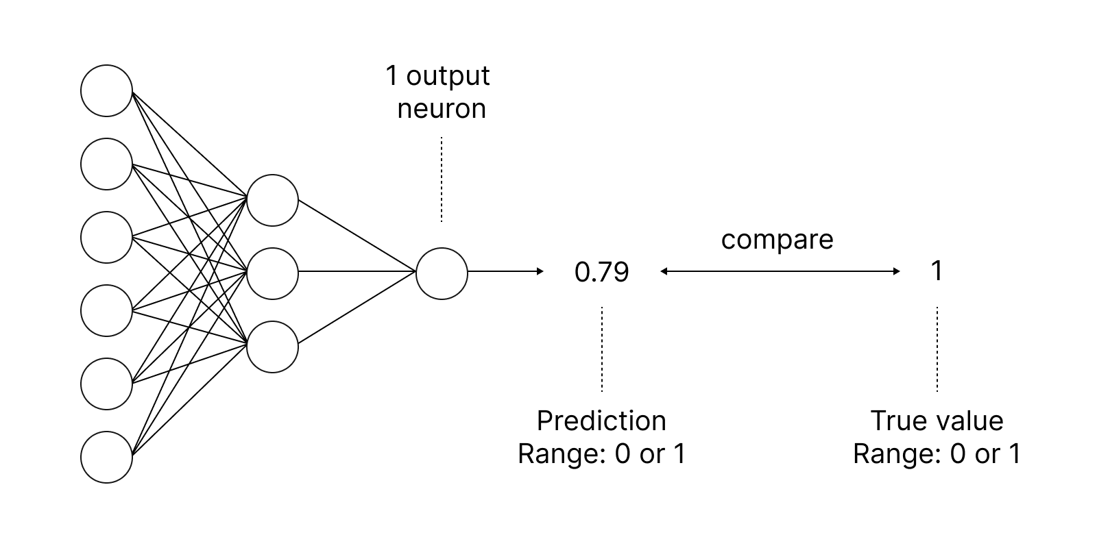
One of the most popular activation functions is the sigmoid.

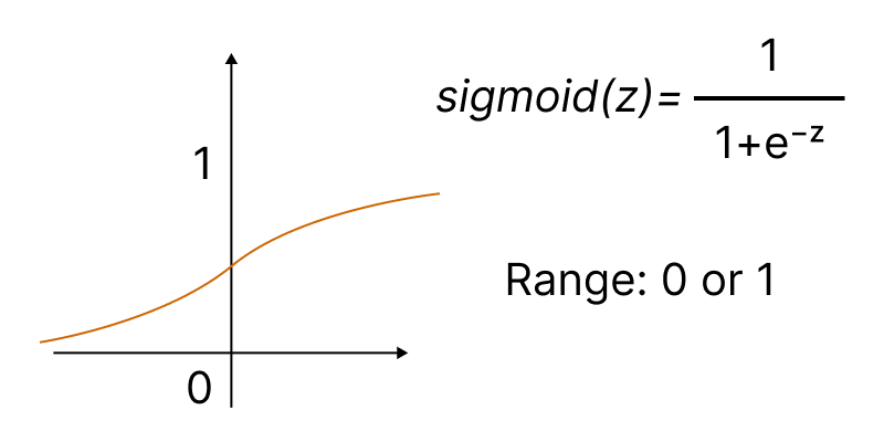
The built-in Activation method allows setting one of the fifteen types of the activation function. All of them are available in the ENUM_ACTIVATION_FUNCTION enumeration.

ID	Description
AF_ELU	Exponential Linear Unit
AF_EXP	Exponential
AF_GELU	Gaussian Error Linear Unit
AF_HARD_SIGMOID	Hard Sigmoid
AF_LINEAR	Linear
AF_LRELU	Leaky Rectified Linear Unit
AF_RELU	Rectified Linear Unit
AF_SELU	Scaled Exponential Linear Unit
AF_SIGMOID	Sigmoid
AF_SOFTMAX	Softmax
AF_SOFTPLUS	Softplus
AF_SOFTSIGN	Softsign
AF_SWISH	Swish
AF_TANH	The hyperbolic tangent function
AF_TRELU	Thresholded Rectified Linear Unit

A neural network aims at finding an algorithm that minimizes the error in learning, for which the loss function is used. The deviation is computed using the Loss method for which you can specify one of fourteen types from the ENUM_LOSS_FUNCTION enumeration.

The resulting deviation values are then used to refine the neural network parameters. This is done using the Derivative method, which calculates the values of the derivative of the activation function and writes the result to the passed vector/matrix. The neural network training process can be visually represented using the animation from the article "Programming a Deep Neural Network from Scratch using MQL Language".

Improvements in OpenCL

We have also implemented matrix and vector support in the CLBufferWrite and CLBufferRead functions. Corresponding overloads are available for these functions. An example for a matrix is show below.

Writes values from the matrix to the buffer and returns true on success.

uint  CLBufferWrite(
   int           buffer,                    // OpenCL buffer handle
   uint          buffer_offset,             // offset in the OpenCL buffer in bytes
   matrix<T>     &mat                       // matrix of values to write to buffer
   );

Reads an OpenCL buffer to a matrix and returns true on success.

uint  CLBufferRead(
   int           buffer,                    // OpenCL buffer handle
   uint          buffer_offset,             // offset in the OpenCL buffer in bytes
   const matrix& mat,                       // matrix to get values from the buffer
   ulong         rows=-1,                   // number of rows in the matrix
   ulong         cols=-1                    // number of columns in the matrix
   );

Let's consider the use of new overloads using an example of a matrix product of two matrices. Let's do the calculations using three method:

A naive way illustrating the matrix multiplication algorithm
The built-in MatMul method
Parallel calculation in OpenCL

The obtained matrices will be checked using the Compare method that compares the elements of two matrices with the given precision.

#define M       3000      // number of rows in the first matrix
#define K       2000      // number of columns in the first matrix equal to the number of rows in the second one
#define N       3000      // number of columns in the second matrix
 
//+------------------------------------------------------------------+
const string clSrc=
  "#define N     "+IntegerToString(N)+"                              \r\n"
  "#define K     "+IntegerToString(K)+"                              \r\n"
  "                                                                  \r\n"
  "__kernel void matricesMul( __global float *in1,                   \r\n"
  "                           __global float *in2,                   \r\n"
  "                           __global float *out  )                 \r\n"
  "{                                                                 \r\n"
  "  int m = get_global_id( 0 );                                     \r\n"
  "  int n = get_global_id( 1 );                                     \r\n"
  "  float sum = 0.0;                                                \r\n"
  "  for( int k = 0; k < K; k ++ )                                   \r\n"
  "     sum += in1[ m * K + k ] * in2[ k * N + n ];                  \r\n"
  "  out[ m * N + n ] = sum;                                         \r\n"
  "}                                                                 \r\n";
//+------------------------------------------------------------------+
//| Script program start function                                    |
//+------------------------------------------------------------------+
void OnStart()
 {
//--- initialize the random number generator
  MathSrand((int)TimeCurrent());
//--- fill matrices of the given size with random values
  matrixf mat1(M, K, MatrixRandom) ;    // first matrix
  matrixf mat2(K, N, MatrixRandom);     // second matrix
 
//--- calculate the product of matrices using the naive way
  uint start=GetTickCount();
  matrixf matrix_naive=matrixf::Zeros(M, N);// here we rite the result of multiplying two matrices
  for(int m=0; m<M; m++)
    for(int k=0; k<K; k++)
      for(int n=0; n<N; n++)
        matrix_naive[m][n]+=mat1[m][k]*mat2[k][n];
  uint time_naive=GetTickCount()-start;   
     
//--- calculate the product of matrices using MatMull
  start=GetTickCount();
  matrixf matrix_matmul=mat1.MatMul(mat2);
  uint time_matmul=GetTickCount()-start;     
  
//--- calculate the product of matrices in OpenCL
  matrixf matrix_opencl=matrixf::Zeros(M, N);
  int cl_ctx;             // context handle
  if((cl_ctx=CLContextCreate(CL_USE_GPU_ONLY))==INVALID_HANDLE)
   {
    Print("OpenCL not found, exit");
    return;
   }
  int cl_prg;             // program handle
  int cl_krn;             // kernel handle
  int cl_mem_in1;         // handle of the first buffer (input)
  int cl_mem_in2;         // handle of the second buffer (input)
  int cl_mem_out;         // handle of the third buffer (output)
//--- create the program and the kernel
  cl_prg = CLProgramCreate(cl_ctx, clSrc);
  cl_krn = CLKernelCreate(cl_prg, "matricesMul");
//--- create all three buffers for the three matrices
  cl_mem_in1=CLBufferCreate(cl_ctx, M*K*sizeof(float), CL_MEM_READ_WRITE);
  cl_mem_in2=CLBufferCreate(cl_ctx, K*N*sizeof(float), CL_MEM_READ_WRITE);
//--- third matrix - output
  cl_mem_out=CLBufferCreate(cl_ctx, M*N*sizeof(float), CL_MEM_READ_WRITE);
//--- set kernel arguments
  CLSetKernelArgMem(cl_krn, 0, cl_mem_in1);
  CLSetKernelArgMem(cl_krn, 1, cl_mem_in2);
  CLSetKernelArgMem(cl_krn, 2, cl_mem_out);
//--- write matrices to device buffers
  CLBufferWrite(cl_mem_in1, 0, mat1);
  CLBufferWrite(cl_mem_in2, 0, mat2);
  CLBufferWrite(cl_mem_out, 0, matrix_opencl);
//--- start the OpenCL code execution time
  start=GetTickCount();
//--- set the task workspace parameters and execute the OpenCL program
  uint  offs[2] = {0, 0};
  uint works[2] = {M, N};
  start=GetTickCount();  
  bool ex=CLExecute(cl_krn, 2, offs, works);
//--- read the result into the matrix
  if(CLBufferRead(cl_mem_out, 0, matrix_opencl))
    PrintFormat("Matrix [%d x %d] read ", matrix_opencl.Rows(), matrix_opencl.Cols());
   else
      Print("CLBufferRead(cl_mem_out, 0, matrix_opencl failed. Error ",GetLastError()); 
  uint time_opencl=GetTickCount()-start;   
  Print("Compare computation times of the methods");
  PrintFormat("Naive product time = %d ms",time_naive);
  PrintFormat("MatMul product time = %d ms",time_matmul);
  PrintFormat("OpenCl product time = %d ms",time_opencl);  
//--- release all OpenCL contexts
  CLFreeAll(cl_ctx, cl_prg, cl_krn, cl_mem_in1, cl_mem_in2, cl_mem_out);
 
//--- compare all obtained result matrices with each other 
  Print("How many discrepancy errors between result matrices?");
  ulong errors=matrix_naive.Compare(matrix_matmul,(float)1e-12);
  Print("matrix_direct.Compare(matrix_matmul,1e-12)=",errors);
  errors=matrix_matmul.Compare(matrix_opencl,float(1e-12));
  Print("matrix_matmul.Compare(matrix_opencl,1e-12)=",errors);
/*
   Result: 
   
   Matrix [3000 x 3000] read 
   Compare computation times of the methods
   Naive product time = 54750 ms
   MatMul product time = 4578 ms
   OpenCl product time = 922 ms
   How many discrepancy errors between result matrices?
   matrix_direct.Compare(matrix_matmul,1e-12)=0
   matrix_matmul.Compare(matrix_opencl,1e-12)=0
*/  
 }
//+------------------------------------------------------------------+
//| Fills the matrix with random values                              |
//+------------------------------------------------------------------+
void MatrixRandom(matrixf& m)
 {
  for(ulong r=0; r<m.Rows(); r++)
   {
    for(ulong c=0; c<m.Cols(); c++)
     {
      m[r][c]=(float)((MathRand()-16383.5)/32767.);
     }
   }
 }
//+------------------------------------------------------------------+
//| Release all OpenCL contexts                                      |
//+------------------------------------------------------------------+
void CLFreeAll(int cl_ctx, int cl_prg, int cl_krn,
               int cl_mem_in1, int cl_mem_in2, int cl_mem_out)
 {
//--- release all created OpenCL contexts in reverse order
  CLBufferFree(cl_mem_in1);
  CLBufferFree(cl_mem_in2);
  CLBufferFree(cl_mem_out);
  CLKernelFree(cl_krn);
  CLProgramFree(cl_prg);
  CLContextFree(cl_ctx);
 }

A detailed explanation of the OpenCL code from this example is provided in the article "OpenCL: From naive towards more insightful coding".

More improvements

Build 3390 lifted two restrictions in OpenCL operation which affected the GPU usage.

The maximum number of OpenCL objects can be up to 65536, while previously there was a limit of 256. OpenCL object handles are created in an MQL5 program using the CLContextCreate, CLBufferCreate and CLProgramCreate function. The previous limit of 256 handles was not enough for the efficient use of machine learning methods.

OpenCL can also be used on graphical cards without 'double' support. Previously, only GPUs supporting double were allowed in MQL5 programs, although many tasks allow calculations using float. The float type is initially considered native for parallel computing, as it takes up less space. Therefore, the old requirement has been lifted.

To set the mandatory use of GPUs with double support for specific tasks, use the CL_USE_GPU_DOUBLE_ONLY in the CLContextCreate call.

   int cl_ctx;
//--- initialization of OpenCL context
   if((cl_ctx=CLContextCreate(CL_USE_GPU_DOUBLE_ONLY))==INVALID_HANDLE)
     {
      Print("OpenCL not found");
      return;
     }

Although changes in OpenCL operations are not directly related to matrices and vectors, they are in line with our efforts in developing the MQL5 language machine learning capabilities.

The future of MQL5 in Machine Learning

Over the past years, we have done a lot to introduce advanced technologies into the MQL5 language:

Porting the ALGLIB library of numerical methods to MQL5
Implementing a mathematical library with fuzzy logic and statistic methods
Introducing the graphics library, analogue of the plot function
Integrating with Python to run Python scripts directly in the terminal
Adding DirectX functions to create 3D graphics
Implementing native SQLite support for operations with data bases
Adding new data types: matrices and vectors, along with all the necessary methods

The MQL5 language will continue to develop, while one of the top priority direction is machine learning. We have big plans for further development. So, stay with us, support us, and keep learning with us.