Regression Analysis of the Influence of Macroeconomic Data on Currency Prices Fluctuation
Salavat Bulyakarov | 19 September, 2014
Introduction
Fundamental analysis is deemed incomprehensible by many. It is unclear how to carry it out, which parameters to take into account and which not to. Finding out the impact of the accounted parameters and the length of time it is to be considered for is not simple either.
In 2011 I came across the article Multiple Regression Analysis. Strategy Generator and Tester in One and found the method described there interesting. I have conducted research on the application of this method to the fundamental analysis and describe the results in this article.
What is 'Multiple Regression Analysis'?
Multiple regression analysis is a method of estimating dependence of one variable from two or more independent variables.
Those of a non-mathematical mind, probably, will not find this definition understandable. The following example is going to illustrate the meaning of the analysis and how it can be used.
Imagine a researcher who is going to estimate the efficiency of regular physical activity when taking a diet supplement. The researcher conducts an experiment involving 24 university students. The students are divided into four groups of six people each. The first group get 100 mg/day of supplement, the second group get 200 mg/day, the third get 300 mg/day, and the forth - 400 mg/day. This experiment involves four levels of supplement intake and three levels of physical activity. Six people in each group are divided into three couples. One couple exercises zero hours a week, the second couple exercises five hours a week and the third one has ten hours of physical activity a week. In the end of the experiment every participant lost weight. The data was entered into the following table:
| Participant of the experiment | Doze of supplement (mg/day) | Level of physical activity (hours/week) | Weight loss (lb) |
|---|---|---|---|
| 1 | 100 | 0 | -4 |
| 2 | 100 | 0 | 0 |
| 3 | 100 | 5 | -7 |
| 4 | 100 | 5 | -6 |
| 5 | 100 | 10 | -2 |
| 6 | 100 | 10 | -14 |
| 7 | 200 | 0 | -5 |
| 8 | 200 | 0 | -2 |
| 9 | 200 | 5 | -5 |
| 10 | 200 | 5 | -8 |
| 11 | 200 | 10 | -9 |
| 12 | 200 | 10 | -9 |
| 13 | 300 | 0 | 1 |
| 14 | 300 | 0 | 0 |
| 15 | 300 | 5 | -3 |
| 16 | 300 | 5 | -3 |
| 17 | 300 | 10 | -8 |
| 18 | 300 | 10 | -12 |
| 19 | 400 | 0 | -5 |
| 20 | 400 | 0 | -4 |
| 21 | 400 | 5 | -4 |
| 22 | 400 | 5 | -6 |
| 23 | 400 | 10 | -9 |
| 24 | 400 | 10 | -7 |
Weight loss result of every participant
Consequently, we have two questions:
- What caused the weight loss - supplements or physical activity?
- What kind of a relationship is there between the change in weight and the influencing factor?
It is very similar to a common situation on financial markets, isn't it? For example, when currency price changes, there is always a question which item of news influenced it. If there is such an economic factor impacting a price, then how does the price change when the factor is varied?
Multiple regressive analysis and the program STATISTICA help to answer those questions. Transfer or import the tables containing data to the program and select 'Multiple Regression' in the menu:

Fig. 1. Import data of the example to the program STATISTICA
After selecting this menu bar, find the button 'Variables' and click on it:
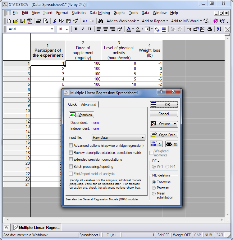
Fig. 2. Multiple analysis parameters screen
It will bring up a window for selecting variables used for analysis. It consists of two parts: on the left hand side we can select what, we believe, is a dependent variable (in our case it is weight loss) and on the right hand side, we highlight what can influence this change.
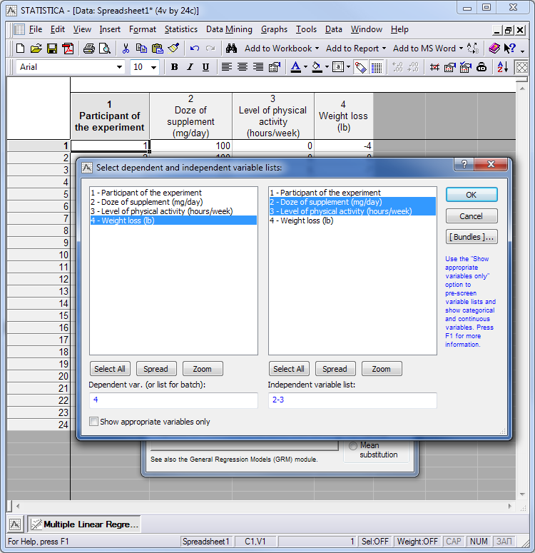
Fig. 3. Assigning dependent and independent variables
Pressing 'OK' will take us back to the previous settings dialog window where we have to tick a check box and then press 'OK':
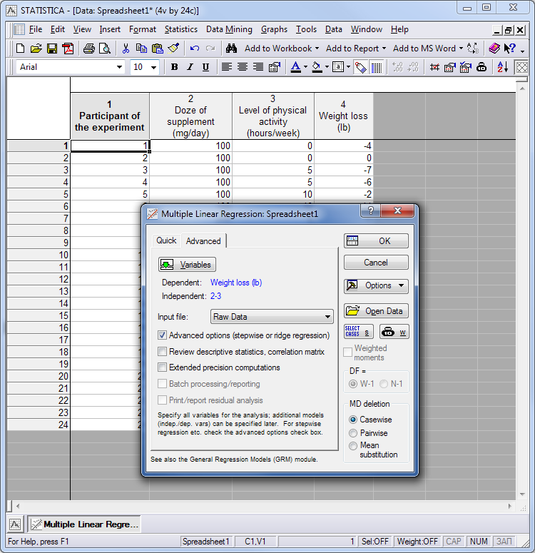
Fig. 4. Selecting parameters for multiple analysis
In the following window we select the method 'All Effects':
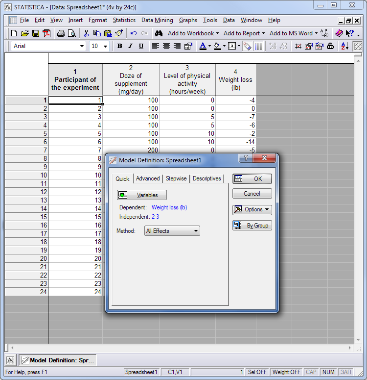
Fig. 5. Select method
After all the manipulations we shall receive a window with the analysis result. Those factors that were statistically proven to influence the result are in red font in the list of factors (in our case it is the 'Level of physical activity'). Other variables:
- 'No. of cases" is a number of incidents for analysis;
- "p" is the level of statistic validity of this correlation (level below 0.05 is believed reliable);
- "Multiple R" is the value of multivariable correlation between the dependent and independent variables of the equation.
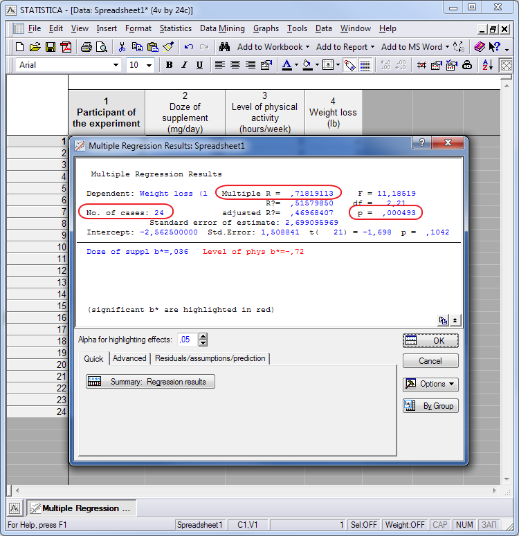
Fig. 6. Data processing result
Value 'Multiple R= 0,71819113' should be interpreted as: 'Multiple R, the value of multivariable correlation between weight loss and factors impacting it, is 71,82%'.
One of two factors, 'Level of Physical Activity', is in red text. It is the factor that affected the weight loss when the impact of taking the diet supplement was insignificant.
Now we only have to calculate how exactly the factors influenced the weight loss by making a tentative regressive equation. To do that, press the button 'Summary: Regression results' for bringing up a new table. Use the values from the column 'b' of this table to make a regression equation:
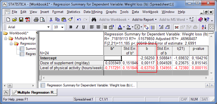
Fig. 7. Variables of regression equation
We got the following equation:
Putting values into the equation (Ctrl+C в STATISTICA -> Ctrl+V в Excel), we can calculate the change in weight if the supplement intake or intensity of physical exercises get different. For example:
- Weight change 1 = 0.00117*100 - 0.6375*0 - 2.5625 = -2,4455. It means that one can lose up to 2.4 lb when taking 100 mg a day and doing no exercises at all.
- Weight change 2 = 0.00117*100 - 0.6375*10 - 2.5625 = -8,8205. That means that the weight loss can be up to 8,82 lb when taking 100 mg of the supplement a day and exercising 10 hours a week.
I hope that this example gives a clear idea what multiple analysis can be used for. Actually, someone might find it useful for checking if their diet is efficient and if they need to go to the gym more.
Now we are going to apply the idea of the experiment to currencies. Let us assume that the dependent variable is a price change of the pair EURUSD and independent variables are the macroeconomic statistics, received from the events calendar of the popular resource Forex Factory.
Similar to the above example, we can identify the macroeconomic factors influencing currency prices through multiple analysis. We can also make an equation that estimates what the value of the currency price will be after macroeconomic statistics get published.
Preparing Data and Importing it to the Program STATISTICA
Working with Forex Factory website, I encountered the following issue that I strongly recommend to consider. On this resource, the same data gets published in different formats. For example, numbers may have a text format or additional text data which makes it difficult to collect data as normal. Parsing the website to gather data may fail.
I manually gathered the values of all 99 factors of the news calendar concerning the USA for the past several years
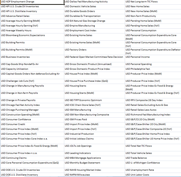
Fig. 8. Published macroeconomic indices of the USA
I processed all numbers to a unified format, deleted all additional text data such as "million" and "billion" etc. and brought all data to a table of seven columns (see the file 'calendar_usd.zip' attached to the article) and added quotes for EURUSD of the D1 period.
Column headers:
- Date
- MonthYear
- Time
- Time Zone
- Currency
- Description
- Previous
The result list has more than 6700 entries of macroeconomic data and quotes for EURUSD and is of no practical use for a simple manual analysis. Bringing all the data into a table where it got sorted in separate columns by the type and arranged in lines by date required an additional handler. We used the script ListConvertToTable to process data and convert it into a table.
In the settings dialog window of the script it is required to name an input file and the target document. The input file has to be initially placed in terminal_data_directory/MQL5/Files, the output one is created there too.
As there is a lot of data, processing of the list of news to a table can take quite a long time. Alerts, built-in in the script, will indicate what stage it is at. Alert '8' will let you know when the process is complete and you can work on the file. The table that will undergo a multiple analysis is in the file attached to this article.
I got the following result (see the file 'calendar_usd_out.zip' in the attachment):
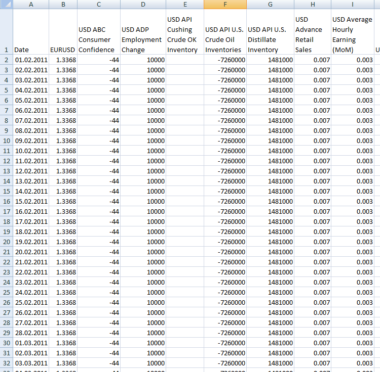
Fig. 9. Result of ListConvertToTable script execution
We shall use the program STATISTICA again to process data. To upload a CSV file to STATISTICA, follow the steps below:
- In STATISTICA open 'File', then 'Open', choose file type 'Data files' and open your CSV file.
- In the window Text File Import Type leave 'Delimited' and press 'OK'.
- In the open window include the underscored items
- In the field 'Decimal separator character' a dot must be placed no matter whether there is one or not:
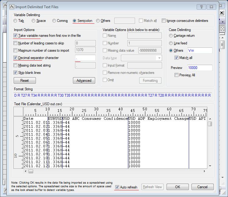
Fig. 10. Importing a table of the .csv format to the program STATISTICA
Press 'OK' and you will receive a table with your data. Data is ready for the multiple regression analysis. To analyze the impact of the data on the following price change, it is necessary to add the periods when the price change took place. I selected the news since 2010 and three options of the dependent variable for analysis:
- Currency price change 1 day after the news was published;
- Currency price change 5 days after the news was published;
- Currency price change 10 days after the news was published.
These columns can be added manually to the CSV table before the export to the program STATISTICA or in the table of the program window:
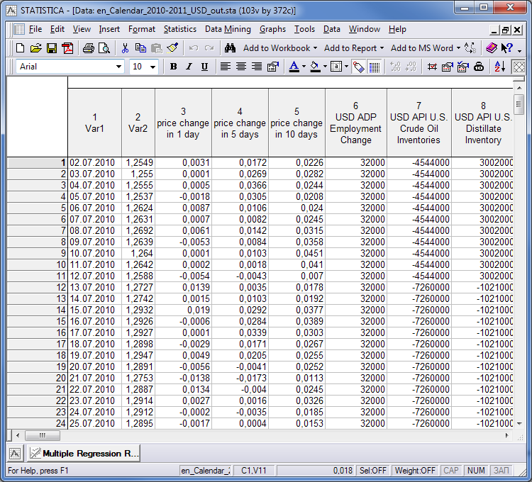
Fig. 11. Extended data table
The data is ready and the indicators that, in our view, affect currency rate can be elicited.
Elicit Factors that Have a Great Impact on Currency Price
Start regression analysis ('Statistics'->'Multiple Regression'). In the appeared window enable the marked items in the tab 'Advanced'. Press the button 'Variables'.
In the first field select the dependent variable and in the second field select independent ones. Our equation will be based on the values of the selected variables:
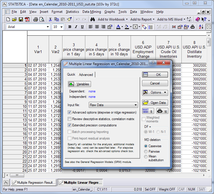
Fig. 12. Window for selecting indicators
Using the button 'Variables', select data to be used for analysis:
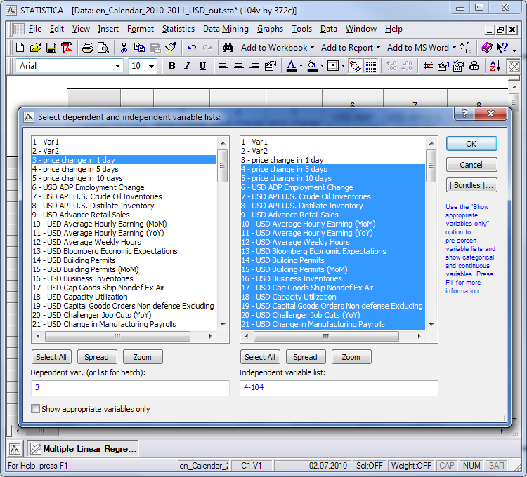
Fig. 13. Assigning dependent and independent variables
A warning window with the sign 'Some variables have no variance' will appear to inform that some selected independent variables cannot be changed without data. Such columns must be deleted. Through elimination we shall find column 49 'USD Federal Open Market Committee Rate Decision', delete it and receive a table ready for analysis (see the file "calendar_2010-2011_usd_out.zip" in the attachment).
Click "OK". In the opened window we tick the check boxes in the 'Advanced' tab:
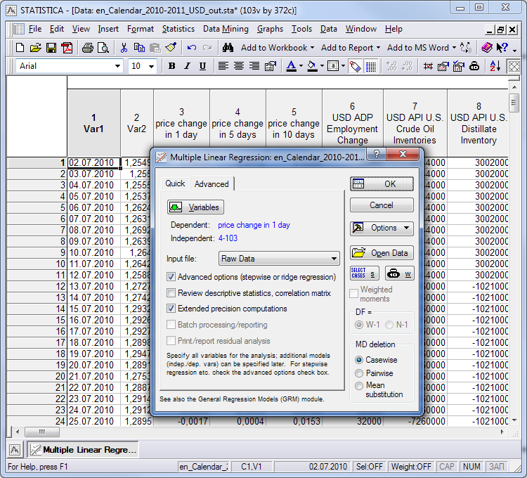
Fig. 14. Select method Forward Stepwise
Complete selecting options by pressing button 'ОK'. In the next window choose method 'Forward Stepwise' to enable automatic data selection and then press 'ОK' again:
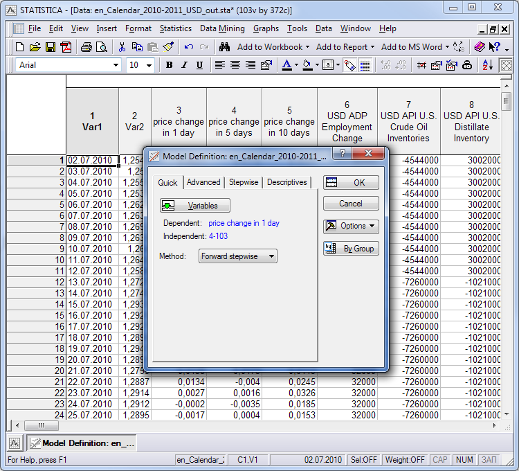
Fig. 15. Select method Forward Stepwise
We are on the homestretch. When you see a message in a new window informing that regression analysis was successful, press the button 'Summary: Regression results'.
Automatic selection of indicators sorts out those making the greatest contribution to the multivariable correlation between independent variables and the dependent one. In our case it is a set of indicators that has the greatest impact on the price. Automatic selection, in essence, has a role of a strategy generator. The generated equation will include only those indicators that describe the behavior of the price the most reliable way.
I must mention though that the rules of including indicators into the analysis used in STATISTICA are not always optimal. For instance, the regression equation can include a lot of non-reliable indicators (black font in the table of result). If the list includes non-reliable indicators, then return to the stage of selecting the indicators and remove the non-reliable ones from the lot, intended for analysis.
To return press 'Cancel' in the window of analysis result and repeat the analysis. Try to exclude all non-reliable indicators this way. At the same time, keep in mind that the obtained value of the multivariable correlation (Multiple R) is not supposed to be significantly less than the initial one. You can remove all non-reliable indicators from the analysis one by one or do them all together. The first method is preferable though.
In the end, only reliable indicators affecting the price fluctuation are meant to stay in the table. In the tables, the variables that were found out to influence the prices were highlighted red and the variables having zero affect are in black.
Upon completion of analysis, some indicators were discovered to have an impact on the currency price after their publication. A set of the indicators was different for each period. Choosing 'price change in 1 day' (i.e. we analyze the behavior of the price in a day after the indicator was published) as an independent variable in the left hand side window, we will receive the following:
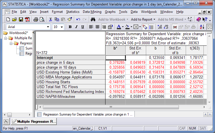
Fig. 16. Independent variable 'price change in 1 day'
Return by clicking 'Cancel' and then select 'Variables' to get back to the lists of variable to choose from. Gradually we remove the entries in black from the list of independent variables and leave only the ones in red. The remaining entries will contain the news affecting the prices in the following day.
Please note that entries in the table differ in color. The independent variables that have a significant impact on the dependent one are in red. At the figure below all entries are in red, i.e. the errors in the equation results after inputting the data will be less than in the first case. The impact can be assessed by the value of the coefficients of the last column 'p-value' (the smaller the value, the better). The variables that have zero impact on the price can be removed based on the coefficients.
Choosing 'price change in 5 days' and sorting out meaningful news by gradually removing irrelevant entries, we shall receive the following result:
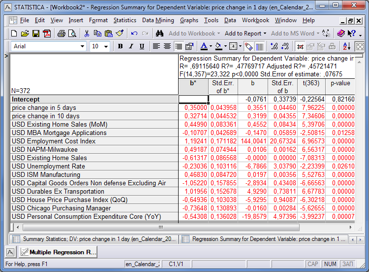
Fig. 17. Independent variable 'price change in 5 days'
When we, finally, select 'price change in 10 days' as an independent variable, we will get:
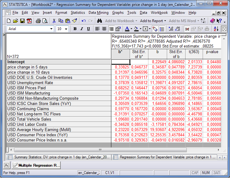
Fig. 18. Independent variable 'price change in 5 days'
When we select as an independent variable the price change in one day after the indicator figures were published, we can see that in the period from 2010 till the middle of 2011 the prices were affected mostly by the data on the sphere of real estate development and indices, published by the Richmond Institute.
In the stretch of 5 days after the data was published, indices of production and non-production industries, labor costs and unemployment figures are added to the data on the development industry.
When we consider 10 days, the breakdown of influential indices changes. Indices of production and non-production industries, applications for house development, unemployment level and energy prices come to the forefront.
Thus, factors, affecting the price of EURUSD pair, are very similar to the macroeconomic data of fundamental analysis, importance of which is emphasized in nearly every textbook. As we can see, it was proved by mathematics and statistics.
Regression Equation and Resulting Forecast
It is not enough to know the factors affecting the price, it is important to be able to estimate how the prices could change at the indice publication. For that we shall make a regression equation like in the example at the beginning of this article.
We shall make a regression equation based on the gathered data from the table of fig. 17 'price change in 5 days'. For that we shall use the variables from the column with the header 'b'. The first line is a numeric constant, received in the end of the analysis. Its calculation will be considered in the following articles.
Let us make a regression equation based on these coefficients:
where we use the values from the column "b" as coefficients and published macroeconomic data as the multipliers of the square brackets.
Inputting the values of macroeconomic indices, published at the source web site, into this equation, we shall receive a number R, greater or less than zero. If the result of inputting new data is greater than zero, then it means that the prices are going to increase within the period, selected for analysis. The value of R will show the price growth. Negative R means that the prices can come down. The value of the R in this case will show the price fall.
Put the values in the above formula and consider the result based on the example of EURUSD. We shall use the data of the entry for 04.08.2010 as an example for putting coefficients into the equation:
| b | value | [b]х[value] | |
|---|---|---|---|
| Intercept | -0.0761 | 1.00000 | -0.0761 |
| price change in 1 day | 0.3551 | -0.0070 | -0.0025 |
| price change in 10 days | 0.3199 | 0.0244 | 0.0078 |
| USD Existing Home Sales (MoM) | 0.4552 | -0.022 | -0.0100 |
| USD MBA Mortgage Applications | -0.1470 | -0.044 | 0.0065 |
| USD Employment Cost Index | 144.0041 | 0.006 | 0.8640 |
| USD NAPM-Milwaukee | 0.0106 | 59 | 0.6278 |
| USD Existing Home Sales | 0.0000 | 5660000 | -0.6596 |
| USD Unemployment Rate | -6.7866 | 0.099 | -0.6719 |
| USD ISM Manufacturing | 0.0197 | 56.2 | 1.1052 |
| USD Capital Goods Orders Non defense Excluding Air | -2.8934 | 0.048 | -0.1389 |
| USD Durables Ex Transportation | 4.9290 | 0.012 | 0.0591 |
| USD House Price Purchase Index (QoQ) | -5.9295 | -0.018 | 0.1067 |
| USD Chicago Purchasing Manager | -0.0160 | 59.1 | -0.9433 |
| USD Personal Consumption Expenditure Core (YoY) | -19.8579 | 0.015 | -0.2979 |
| -0.0230 |
R=-0,0230, therefore a downtrend continued for the following five days starting from 04.08.2010 and the price dropped down to -230 points. Let us take a look at the chart of the EURUSD pair for this period:
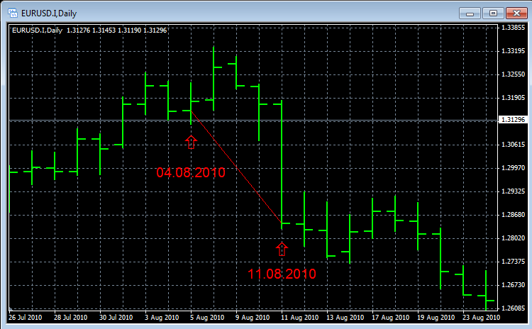
Fig. 19. EURUSD august 2010
As we can see from the chart, the forecast was accurate and the price dropped from 1.3154 to 1.2844 in five trading days (closing on the 11th of August), i.e. -310 points. The forecast for the price drop based on the result of the regression equation was proven. Similarly, other dates can be put in.
Conclusion
A way of analyzing data on macroeconomic indicators considered in this article, allows simplifying and automating fundamental analysis so even a novice can handle vast amount of economic statistics.
Moreover, such an approach to fundamental analysis gives an opportunity to react instantly and adjust deals according to news.
Please be aware though that the forecast should not be deemed as an absolute guarantee that the currency price will be changing in the predicted direction. The forecast result is probabilistic and depends on a lot of factors. Besides, the regression equation needs to be recalculated when new data comes out.
Good luck with your forecasts!