Technical Indicators and Digital Filters

Introduction

For several years, Code Base has accumulated a large number of indicators. Many of them are copies of one another with only slight modifications. After many hours of visual comparison of indicators on the chart, we could not help but ask: "Is it possible to find more objective and efficient way of comparison?" It is possible, indeed. We should admit that an indicator is a digital filter. Let's turn to Wikipedia.

Filter (chemistry), a device (usually a membrane or layer) that is designed to physically block certain objects or substances while letting others through.

Do you agree that indicators allow blocking some "unnecessary" objects and focus on the critical ones? Now let's see what a digital filter is.

In electronics, computer science and mathematics, a digital filter is a system that performs mathematical operations on a sampled, discrete-time signal to reduce or enhance certain aspects of that signal.

In other words, a digital filter is a filter processing discrete signals. The prices we see in the terminal can be treated as discrete signals, as their values are recorded not continuously but over a certain period of time. For example, the price value is recorded each hour on H1 chart, while it is done once per 5 minutes on M5. Many indicators can be treated as linear filters. This is exactly the type of indicators that are discussed in the present article. 

Now, when we found out that we are dealing with digital filters, let's examine the theory in order to define what parameters should be compared.

1. Frequencies and Periods

First of all, I should mention that any curve can be represented as a sum of sine waves.

Vibration period is the time interval between two successive passes of a body via the same position and in the same direction. This value is reciprocal to frequency.

This definition can be most easily understood by using a sine wave. Let's consider a period equal to 10 counts. We will perform calculation in bars for simplicity.

 

 Fig. 1. Sample periodic signal

As we can see, the line completes the entire cycle within 10 counts, while the eleventh bar is the first point of the new cycle.

What is the frequency of the sine wave? The definition states that period is a value reciprocal to frequency. Then, if the period is equal to 10 (bars), the frequency will be 1/10=0.1 (1/bars).

In physics, periods (T) are measured in seconds (s), while frequencies (f) - in Hertz (Hz). If we are dealing with a minute time frame, then T=60*10=600 seconds, while f=1/Т=1/600=0.001667 Hz. Herz and seconds are used mostly in analog filters. In digital ones, counts are usually used (in the way we used bars). If necessary, they are multiplied by the necessary amount of seconds.

You may wonder, what this has to do with sine waves? Sine waves are necessary to explain the physical meaning of filters and moving to frequencies, as this concept is used in the appropriate works. Now, let's take 7 sine waves instead of one with periods from 10 to 70 and a step of 10 bars. Bars in the upper subwindow on Fig. 2 serve as a guide to visually estimate the number of counts.

 

 Fig. 2. Seven sine waves having the same amplitude with periods of 10, 20, ... 70 bars.

The scale is large enough but it is still possible to get confused. And it is much easier to get confused, if we have much more sine waves.

The sum of sine waves is displayed below:

  

Fig. 3. The sum of seven sine waves shown in Fig. 2

The frequencies are shown in the following way:

  

Fig. 4. The spectrum of sine waves' sum  (in frequencies)

7 counts are enough for displaying 7 sine waves. Pay attention to the colors, they correspond to the previous figure. Slow sine waves are followed by fast ones. The lowest possible frequency is 0 (constant component), while the highest one is 0.5 (1/bars). The case will be the opposite for periods.

 

 Fig. 5. The spectrum of sine waves' sum (in periods)

We remember that the frequency is equal to 1/period. Therefore, the period should be within the range of 2 up to infinity. Why 0.5 and 2? One sine wave can be described by at least two counts (see Nyquist–Shannon sampling theorem). To restore the analog (continuous) signal, we need two or more counts per one sine wave (0.5 is received from 1/2).

Let's consider the following table to avoid confusion with periods and frequencies:

Period		100	50	16	10	4	2
Frequency	0	0.01	0.02	0.0625	0.1	0.25	0.5

 

We have examined the concepts of period and frequency, as these are the basic things. All further information is associated with these terms.

 

2. Digital Filters

So, we are finally ready to discuss the filters. Suppose that we have to remove the sine waves having a period less than 50.

 

 Fig. 6. Slow (low frequency) components of sine waves' sum (periods of 50, 60 and 70 bars)

It is all comparatively easy when we know initial components. But what if we know only the sum? In this case, we need a low-pass filter (LPF) with a cut-off frequency of 1/45 (1/bars).

Filtration result will look as follows:

 

 Fig. 7. Result of sine waves' sum filtration (blue line) using LPF

Now, let's leave only the sine wives having the periods of 10, 20 and 30. To do this, we should use a high-pass filter (HPF) with a cut-off frequency of 1/35 (1/bars). 

 

 Fig. 8. High frequency components of sine waves' sum (periods of 10, 20 and 30 bars)

 

Fig. 9. Result of sine waves' sum filtration (blue line) using HPF

To leave the periods of 30, 40 and 50, we need a bandwidth filter (BF) with cut-off frequencies of 1/25 and 1/55 (1/bars). 

 

 Fig. 10. Sine lines having periods of 30, 40 and 50 bars

 

 

Fig. 11. Result of sine waves' sum bandwidth filtration (30-50 bars)

If we want to remove the periods of 30, 40 and 50, we need a band-stop (rejection) filter with the same cut-off frequencies 1/25 and 1/55 (1/bars). 

 

Fig. 12. Sine waves with the periods of 10, 20, 60 and 70 bars

 

 

Fig. 13. The result of rejection filter operation (30-50 bars) depending on the sine waves' sum

Let's sum up the intermediate results in the image below: 

 

Fig. 14. Frequency parameters of the ideal filters: lower frequencies (LPF), upper frequencies (HPF), bandwidth (BF) and rejection (RF) ones

The filters examined above are idealized. Reality is much more different.

  

Fig. 15. Transition band in filters

There is a transition band between acceptance and attenuation bands. Its slope is measured in dB/octave or dB/decade. Octave is a segment between the frequency random value and its double value. Decade is a segment between the frequency random value and its tenfold value. Formally, the transition band is located between the cut-off frequency and attenuation band. Looking ahead, I should say that the cut-off frequency by the spectrum is most often defined by the level of 3 dB.

Outband rejection is suppression of frequencies in the attenuation band measured in decibels.

The beats are detected in the acceptance band. As we are dealing with real filters, i.e., distortions at the acceptance band, some frequencies are greater by their amplitude, while some are lower. The value is measured in decibels.

The table below can help you to render the value in dB:

dB	Amplitude ratio
0.5	1.06
1	1.12
3	1.41
6	2
10	3.16
20	10
30	31.6
40	100
60	1000

 

For example, if we want to receive the result for 60 dB, we can find the values for 20 and 40 dB and multiply them.

Now that we know the basic parameters of the filter, let's turn to the practical part of the article.

3. Searching for the Kernel

We can say that the digital filter is completely described by its impulse response (kernel). Impulse response is a filter's response to a single impulse. The filters can be of IIR (infinite impulse response, for example, Exponential Moving Average, EMA) and FIR (finite impulse response, for example, Simple Moving Average, SMA) types. 

Now, we can focus our attention on MetaEditor. First, let's create a single impulse. It will be a very simple indicator which will display only one count equal to one. In MetaEditor, click New, select "Custom Indicator" and click Next:

 

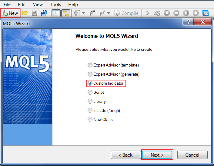
Fig. 16. Creating a custom indicator in MQL5 Wizard

Specify "Impulse" as a name:

 

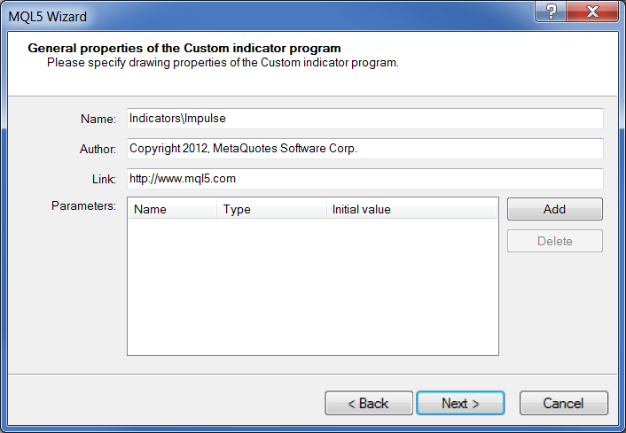
Fig. 17. Indicator's general properties

Select the event handler:

 

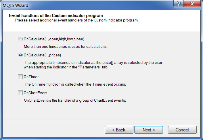
 Fig. 18. Indicator's event handlers

Now, we should add the indicator line and displaying in a separate window. Everything is ready.

 

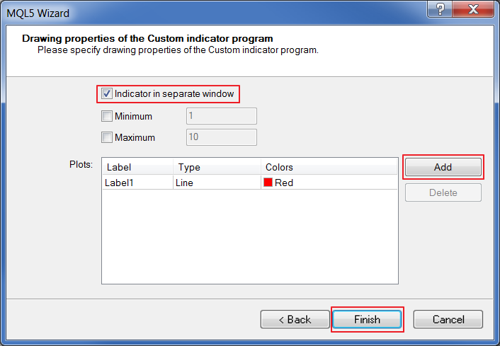
 Fig. 19. Indicator's drawing properties

The indicator's code looks as follows:

//+------------------------------------------------------------------+
//|                                                      Impulse.mq5 |
//|                        Copyright 2012, MetaQuotes Software Corp. |
//|                                              https://www.mql5.com |
//+------------------------------------------------------------------+
#property copyright "Copyright 2012, MetaQuotes Software Corp."
#property link      "https://www.mql5.com"
#property version   "1.00"
#property indicator_separate_window
#property indicator_buffers 1
#property indicator_plots   1
//--- plot Label1
#property indicator_label1  "Label1"
#property indicator_type1   DRAW_LINE
#property indicator_color1  clrRed
#property indicator_style1  STYLE_SOLID
#property indicator_width1  1
//--- input parameters

//--- indicator buffers
double         Label1Buffer[];
//+------------------------------------------------------------------+
//| Custom indicator initialization function                         |
//+------------------------------------------------------------------+
int OnInit()
  {
//--- indicator buffers mapping
   SetIndexBuffer(0,Label1Buffer,INDICATOR_DATA);
   ArraySetAsSeries(Label1Buffer,true);
//---
   return(0);
  }
//+------------------------------------------------------------------+
//| Custom indicator iteration function                              |
//+------------------------------------------------------------------+
int OnCalculate(const int rates_total,
              const int prev_calculated,
              const int begin,
              const double &price[])
  {
//---
   ArrayInitialize(Label1Buffer,0.0);
   Label1Buffer[1023]=1.;
//--- return value of prev_calculated for next call
   return(rates_total);
  }
//+------------------------------------------------------------------+

Add the following to OnInit() function:

ArraySetAsSeries(Label1Buffer,true);

so that the indexing is performed from the end of the array.

In OnCalculate():

ArrayInitialize(Label1Buffer,0.0);
Label1Buffer[1023]=1.;

Let's zero out all the values and add 1 to 1023th indicator's array cell.

Compile (F7) and receive the following result: 

 

 Fig. 20. Impulse indicator

Now, if we apply some indicator, we are able to see its impulse response up to 1024 counts (see Examples).

Of course, it is great to view the filter's kernel but more data can be obtained only from the frequency-domain representation. To do this, we need to create a spectrum analyzer or use a ready-made solution without much effort. Let's select the second option and use SpecAnalyzer indicator described in the article "Building a Spectrum Analyzer".

The indicator is displayed below:

 

Fig. 21. SpecAnalyzer

Some preparatory work is necessary before using it. All necessary steps are described below.

4. Adaptation for Spectrum Analyzer

"External Data" button allows using data from SAInpData indicator.

The original contains the array representing the filter's kernel. We are going to remake the file, so that it is possible to pass any chart indicators to the spectrum analyzer. Automatic and manual modes are to be provided in the modified indicator. In the automatic mode, the first chart indicator to be found is used. In the manual mode, users can set a subwindow and indicator index in the list. In this case, Impulse indicator should be manually added to the chart. After that, the necessary indicator is applied to receive the kernel.

Let's get started. We should create a new indicator following the same algorithm, as with Impulse. Add the input parameters:

input bool Automatic=true; // Autosearch
input int  Window=0;       // Subwindow index
input int  Indicator=0;    // Indicator index

If Automatic=true, the automatic mode is used, while other input parameters are ignored. If Automatic=false, the manual mode with subwindow and indicator index is used.

Next, we should add integer type variables on the global level for storing the handles.

int Impulse=0; // single impulse's handle
int Handle=0;  // required indicator's handle
int Kernel=0;  // filter kernel's handle

Impulse indicator handle is to be stored in Impulse. The handle of the indicator, the kernel of which we want to view in the spectrum analyzer, is to be stored in Handle. The handle of the target indicator, which is built based on Impulse indicator, or, in other words, the target indicator's kernel is to be stored in Kernel.

OnInit() function:

int OnInit()
  {
//--- indicator buffers mapping
   SetIndexBuffer(0,DataBuffer,INDICATOR_DATA);

   Impulse=iCustom(NULL,0,"SpecAnalyzer\\Impulse");//get the single impulse handle
   if(Impulse==INVALID_HANDLE)
     {
      Alert("Impulse initialization failed"); 
       return(INIT_FAILED);
     }
//---
   return(0);
  }

Since Impulse indicator is not changed during the program's operation, the indicator's handle should be received in OnInit() function. Also, handle receiving error should be checked. In case of failure, "Impulse initialization failed" message is displayed and indicator's operation is interrupted with INIT_FAILED key.

OnDeinit() function:

void OnDeinit(const int reason)
  {
//--- delete the indicators
   IndicatorRelease(Impulse);
   IndicatorRelease(Handle);
   IndicatorRelease(Kernel);
  }

Used indicators are deleted in OnDeinit() function.

OnCalculate() function:

static bool Flag=false;        //error flag
if(Flag) return(rates_total); //exit in case of the flag

Flag static variable is added at the beginning of the function. If errors occur during the program's execution, Flag is equal to true and all further iterations of OnCalculate() functions are interrupted right from the start.

Below is the code block associated with the manual mode:

   string Name;  //short name of the required indicator
   if(!Automatic)//in case of the manual mode
     {
      if(ChartIndicatorsTotal(0,Window)>0)//if an indicator is present
        {
         Name=ChartIndicatorName(0,Window,Indicator);//search for its name
         Handle=ChartIndicatorGet(0,Window,Name);//search for the handle
        }
      else//otherwise
        {
         Alert("No indicator");
         Flag=true;
         return(rates_total);
        }

      if(Handle==INVALID_HANDLE)//in case of a handle receiving error
        {
         Alert("No indicator");
         Flag=true;
         return(rates_total);
        }

      CopyBuffer(Handle,0,0,1024,DataBuffer);//display the kernel on the chart
      return(rates_total);
     }

If Automatic=false, the manual mode is launched. The presence of the indicator is checked. In case of success, we start searching for a name and a handle, checking the handle for errors, copying the data to the indicator's buffer. In case of failure, "No indicator" message is displayed, Flag is switched to true, OnCalculate() function execution is interrupted.

The automatic mode block is much more interesting. It consists of searching for an indicator on the chart and creating a kernel.

So, let's consider searching for an indicator. The main objective is to receive a handle.

   if(ChartIndicatorsTotal(0,0)>0)//if the indicator is in the main window
     {
      Name=ChartIndicatorName(0,0,0);//search for its name
      if(Name!="SpecAnalyzer")//if it is not SpecAnalyzer
         Handle=ChartIndicatorGet(0,0,Name);//look for a handle
      else
        {
         Alert("Indicator not found");
         Flag=true;
         return(rates_total);
        }
     }
   else//otherwise
   if(ChartIndicatorsTotal(0,1)>0)//if the indicator is in the first subwindow
     {
      Name=ChartIndicatorName(0,1,0);//search for its name
      if(Name!="SAInpData")//if it is not SAInpData
         Handle=ChartIndicatorGet(0,1,Name);//look for a handle
      else//otherwise
        {
         Alert("Indicator not found");
         Flag=true;
         return(rates_total);
        }
     }

   if(Handle==INVALID_HANDLE)//in case of a handle receiving error
     {
      Alert("No indicator");
      Flag=true;
      return(rates_total);
     }

First, we search for an indicator in the chart's main subwindow and make sure that it is not SpecAnalyzer. If no indicator is found in the main window, we search for it in the next subwindow (considering that there may be SAInpData here). All other actions are similar to the manual mode.

Let's create an indicator. We should receive the parameters of the obtained indicator and create a similar indicator based on Impulse:

   ENUM_INDICATOR indicator_type;//obtained indicator's type
   MqlParam parameters[];      //parameters
   int parameters_cnt=0;      //number of parameters

//--- receive the indicator's type, parameter values and amount
   parameters_cnt=IndicatorParameters(Handle,indicator_type,parameters);
//--- define that a single impulse is to be sent to the indicator's input
   parameters[parameters_cnt-1].integer_value=Impulse;
//--- receive the indicator's handle from the single impulse - filter's kernel
   Kernel=IndicatorCreate(NULL,0,indicator_type,parameters_cnt,parameters);

   if(Kernel==INVALID_HANDLE)//in case of a handle receiving error
     {
      Alert("Kernel initialization failed");
      Flag=true;
      return(rates_total);
     }

   CopyBuffer(Kernel,0,0,1024,DataBuffer);//display the kernel on the chart

indicator_type - the variable of the special enumerated ENUM_INDICATOR type. The variable is designed for receiving the indicator type.

parameters[] - the array of MqlParam type, special structure for storing and transferring the indicator parameters. 

IndicatorParameters function allows receiving data on the chart indicator. Then, we implement slight changes to the parameters' array. Impulse indicator handle is included in the last cell where time series name (close, low, handle, etc.) is stored in the integer_value field. Then, we use IndicatorCreate function to create a new indicator that is also a kernel. Now, we should check the handle and display the kernel on the chart.

SpecAnalyzer indicator has also been slightly changed. The following input parameters have been added:

input bool Automatic=true; //Autosearch
input int Window=0;        //Subwindow index
input int Indicator=0;    //Indicator index

SAInpData call has also been changed:

ExtHandle=iCustom(NULL,0,"SpecAnalyzer\\SAInpData",Automatoc,Window,Indicator);

SAInpData can be used alone to view the impulse response.

 

5. Examples

In order to make things work, paste SpecAnalyzer folder to MetaTrader 5\MQL5\Indicators. Launch MetaTrader 5, open a new EURUSD chart:

Fig. 22. Opening a new EURUSD chart

Now, we apply the necessary indicator, for example, MA(16):

Fig. 23. Applying Moving Average indicator to EURUSD chart

Launch SpecAnalyzer:

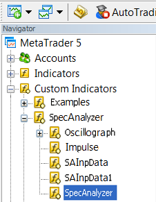
Fig. 24. Launching SpecAnalyzer

Parameters window appears:

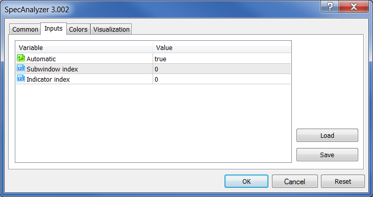
Fig. 25. SpecAnalyzer indicator parameters

For automatic mode, just click OK. In manual mode, true should be replaced to false and the location of a necessary indicator should be specified.

So, we have clicked OK. Click "External Data" in the newly appeared Spectrum Analyzer window:

Fig. 26. Selecting input data for SpecAnalyzer indicator

Now, let's consider working in manual mode. First, we should add Impulse indicator to the chart:

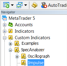
Fig. 27. Adding Impulse indicator

Then, we should use this indicator to generate the target one. To do this, we should drag the indicator by mouse to Impulse window and select the previous indicator data in the "Apply to" field of the parameters:

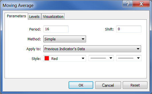
Fig. 28. Generating Moving Average indicator using Impulse indicator data

The following result should be obtained:

 

Fig. 29. Result of Moving Average indicator calculation on a single Impulse

Now, right-click to view the list of indicators:

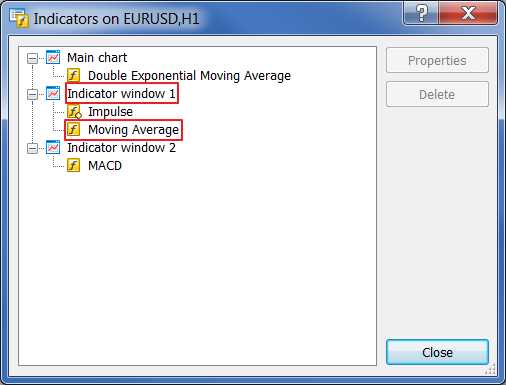
Fig. 30. Indicators in the list

Our indicator is located in subwindow 1 and has the serial number 1 (do not forget that indexing starts from zero, not one). Now, let's launch SpecAnalyzer. Set false, 1, 1. Click "External Data".

The indicator's properties can be changed on the fly. Try to change the period using the indicator list and see how the Spectrum Analyzer responds. 

Before moving on to the examples, it is necessary to mention one feature of SpecAnalyzer indicator. The readings on its scale are not periods but frequency grid marks. The spectrum analyzer works with the kernel having the length of up to 1024 readings. It means that the pitch of the grid frequency is equal to 1/1024=0,0009765625. Thus, the value of 128 on the scale corresponds to the frequency of 0.125 or the period of 8.

Scale	Period
16	64
32	32
64	16
128	8
256	4
384	2.67
512	2

SMA (16)

 

Fig. 31. Simple Moving Average indicator's impulse response (FIR filter)

 

Fig. 32. Simple Moving Average indicator's frequency response

We can see that this is a low-pass filter, as low frequencies prevail. Suppression in the attenuation band is poor.

  

EMA (16)

Fig. 33. Exponential Moving Average indicator's impulse response (IIR filter)

 

Fig. 34. Exponential Moving Average indicator's frequency response

Exponential Moving Average indicator is also a low-pass filter. The line is quite smooth but, unlike the previous indicator, the transition band is wider. Suppression is approximately the same.

Now, let's examine the results of the Universal digital filter.

Low-pass filter

Fig. 35. The impulse response (kernel) of the low-pass filter

Fig. 36. The frequency response of the low-pass filter

High-pass filter

  

Fig. 37. The impulse response (kernel) of the high-pass filter

 

  

Fig. 38. The frequency response of the high-pass filter

 

Band-pass filter

  

Fig. 39. The impulse response (kernel) of the band-pass filter

 

 

  Fig. 40. The frequency response of the band-pass filter

Conclusion

In conclusion, it should be noted that filter parameters are strongly interconnected. Improving some of them implies the deterioration of the others. Therefore, parameters should be selected based on the task at hand.

For example, if you want increased suppression of frequencies in the attenuation band, you need to sacrifice the downward curve's steepness. If both parameters should be good, then we need to increase the kernel's length, which will in turn impact the gap between the indicator and the price or increase distortions in the acceptance band.