Econometric Approach to Analysis of Charts

Theories without facts may be barren, but facts without theories are meaningless.

 K. Boulding

Introduction

I often hear that markets are volatile and there is no stability. And it explains why a successful long-term trading is impossible. But is it true? Let's try to analyze this problem scientifically. And let's choose the econometric means of analysis. Why them? First of all, the MQL community loves precision, which is going to be provided by math and statistics. Secondly, this has not been described before, if I'm not mistaken.

Let me mention that the problem of successful long-term trading cannot be solved within a single article. Today, I'm going to describe only several methods of diagnostics for the selected model, which hopefully will appear valuable for future use.

In addition to it, I'll try my best to describe in a clear way some dry material including formulas, theorems and hypotheses. However, I expect my reader to be acquainted with basic concepts of statistics, such as: hypothesis, statistical significance, statistics (statistical criterion), dispersion, distribution, probability, regression, autocorrelation, etc.

1. Characteristics of a Time Series

It's obvious, that the object of the analysis is a price series (its derivatives), which is a time series.

Econometricians study time series from the point of frequency methods (spectrum analysis, wavelet analysis) and the methods of time domain (cross-correlation analysis, autocorrelation analysis). The reader has already been supplied with the "Building Spectrum Analysis" article that describes the frequency methods. Now I suggest taking a look into the time domain methods, into the autocorrelation analysis and the analysis of conditional variance in particular.

Non-linear models describe the behavior of price time series better than the linear ones. That is why let's concentrate on studying non-linear models in this article.

Price time series have special characteristics that can be taken into account only by certain econometric models. First of all, such characteristics include: "fat tail", clusterization of volatility and the leverage effect.      

                                                                                                                

 

Figure 1. Distributions with different kurtosis.

The fig. 1 demonstrates 3 distributions with different kurtosis (peakedness). Distribution, which peakedness is lower than the normal distribution, has "fat tails" more often than the others. It is shown with the pink color.

We need distribution to show the probability density of a random value, which is used for counting of values of the studied series.

By clusterization (from cluster - bunch, concentration) of volatility we mean the following. A time period of high volatility is followed by the same one, and a time period of low volatility is followed by the identical one. If prices were fluctuating yesterday, most probably they'll do it today. Thus, there is inertia of volatility. The fig. 2 demonstrates that the volatility has a clustered form.

Figure 2. Volatility of daily returns of USDJPY, its clusterization.

The leverage effect consists in the volatility of a falling market is higher than the one of a rising market. It is stipulated by increase of the leverage coefficient, which depends on the ratio of borrowed and own assets, when the share prices fall. Though, this effect applies to the stock market, not the foreign exchange market. This effect won't be considered further.

2. The GARCH Model

So, our main goal is to forecast the exchange rate (price) using some model. Econometricians use mathematical models describing one or another effect that can be estimated in terms of quantity. In simple words, they adapt a formula to an event. And in this way they describe that event.

Considering that the analyzed time series has properties mentioned above, an optimal model that considers these properties will be a non-linear one. One of the most universal non-linear models is the GARCH model. How can it help us? Within its body (function), it will consider the volatility of the series, i.e. the variability of dispersion at different periods of observing. Econometricians call this effect with an abstruse term - heteroscedasticity (from greek - hetero - different, skedasis - dispersion).

If we take a look at the formula itself, we will see that this model implies that the current variability of dispersion (σ²t) is affected by both previous changes of parameters (ϵ²t-i) and previous estimations of dispersion (so called «old news») (σ²t-i):

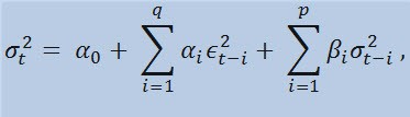
with limits

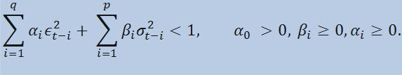
where: ϵt - nonnormalized innovations; α0 , βi , αi , q (order of ARCH members ϵ²), p (order of GARCH members σ²)   -  estimated parameters and the order of models.

3. Indicator of Returns

Actually, we're not going to estimate the price series itself, but the series of returns. The logarithm of price change (constantly charged returns) is determined as a natural logarithm of returns percentage:

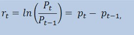
where:

• Pt - is the value of the price series at the time t;
  
• Pt-1 - is the value of the price series at the time t-1;
  
• pt = ln(Pt)  - is the natural logarithm Pt.
  

Practically, the main reason why working with returns is more preferable than working with prices is the returns has better statistical characteristics.

So, let's create an indicator of returns ReturnsIndicator.mq5, which will be very useful for us. Here, I'm going to refer to the "Custom Indicators for Newbies" article that understandably describes the algorithm of creating an indicator. That's why I will show you only the code where the mentioned formula is implemented. I think it's very simple and doesn't require explanation.

//+------------------------------------------------------------------+
//| Custom indicator iteration function                              |
//+------------------------------------------------------------------+
int OnCalculate(const int rates_total,      // size of the array price[]
                const int prev_calculated,  // number of bars available at the previous call
                const int begin,            // index of the array price[] the reliable data starts from
                const double& price[])      // array for the calculation itself

  {
//---
   int start;
   if(prev_calculated<2) start=1;  // start filling ReturnsBuffer[] from the 1-st index, not 0.
   else start=prev_calculated-1;   // set 'start' equal to the last index in the arrays
   for(int i=start;i<rates_total;i++)
     {
      ReturnsBuffer[i]=MathLog(price[i]/price[i-1]);
     }
//--- return value of prev_calculated for next call
   return(rates_total);
  }
//+------------------------------------------------------------------+

The only thing I want to mention is the series of returns is always smaller than the primary series by 1 element. That's why we're going to calculate the array of returns starting from the second element, and the first one will be always equal to 0.

Thus, using the ReturnsIndicator indicator we obtained a random time series that will be used for our studies.

4. Statistical Tests

Now it is the turn of statistical tests. They're conducted to determine if the time series has any signs that prove the suitability of using one or another model. In our case, such model is the GARCH model.

Using the Q-test of Ljung-Box-Pierce, check if the autocorrelations of the series are random or there is a relation. For this purpose, we need to write a new function. Here, by autocorrelation I mean a correlation (probabilistic connection) between the values of the same time series X (t) at the time moments t1 and t2. If the moments t1 and t2 are adjacent (one follows another), then we search for a relation between the members of series and the members of the same series shifted by one time unit: x1, x2, x3, ... и x1+1, x2+1, x3+1, ... Such effect of moved members is called a lag (latency, delay). The lag value can be any positive number.

Now, I'm going to make parenthetic remark and tell you about the following. As far as I know, neither С++, nor MQL5 have standard libraries that cover complex and average statistical calculations. Usually, such calculations are performed using special statistic tools. As for me, it's easier to use tools such as Matlab, STATISTICA 9, etc. to solve the problem. However, I decided to refuse from using external libraries, firstly, to demonstrate the how powerful the MQL5 language is for calculations, and secondly... I learned a lot for myself when writing the MQL code.

Now we need to make the following note. To conduct the Q test, we need complex numbers. That is why I made the Complex class. Ideally, it should be called CComplex. Well, I allowed myself to relax for a while. I'm sure, my reader is prepared and I don't need to explain what a complex number is. Personally, I don't like the functions that calculate the Fourier transformation published at MQL5 and MQL4; complex numbers are used there in an implicit way. Moreover, there is another obstacle - the impossibility of overriding arithmetic operators in MQL5. So I had to look for other approaches and avoid the standard 'C' notation. I have implemented the class of complex number in the following way:

class Complex
  {
public:
   double            re,im; //re -real component of the complex number, im - imaginary
public:
   void              Complex(){};                                   //default constructor
   void              setComplex(double rE,double iM){re=rE; im=iM;}; //set method (1-st variant)
   void              setComplex(double rE){re=rE; im=0;};           //set method (2-nd variant)  
   void              ~Complex(){};                                  //destructor
   void              opEqual(const Complex &y){re=y.re;im=y.im;};   //operator=
   void              opPlus(const Complex &x,const Complex &y);      //operator+   
   void              opPlusEq(const Complex &y);                    //operator+=
   void              opMinus(const Complex &x,const Complex &y);     //operator-
   void              opMult(const Complex &x,const Complex &y);      //operator*   
   void              opMultEq(const Complex &y);                    //operator*= (1-st variant)     
   void              opMultEq(const double y);                       //operator*= (2-nd variant)    
   void              conjugate(const Complex &y);                   //conjugation of complex numbers
   double            norm();                                       //normalization 
 };

For example, the operation of summing two complex numbers can be performed using the method opPlus, subtracting is performed using opMinus, etc. If you just write the code c = a + b (where a, b, с are complex numbers) then the compiler will display an error. But it will accept the following expression: c.opPlus(a,b).

If needed, a user can extend the set of method of the Complex class. For example, you can add an operator of division. 

In addition, I need auxiliary functions that process arrays of complex numbers. That's why I implemented them outside the Complex class not to cycle the processing of array elements in it, but to work directly with the arrays passed by a reference. There are three such functions in total:

1. getComplexArr (returns a two-dimensional array of real numbers from an array of complex numbers);
2. setComplexArr (returns an array of complex numbers from a unidimensional array of real numbers);
3. setComplexArr2 (returns an array of complex numbers from a two-dimensional array of real numbers).
   

It should be noted that these functions return arrays passed by a reference. That's why their bodies do not contain the 'return' operator. But reasoning logically, I think we can speak about the return despite of the void type. 

The class of complex numbers and auxiliary functions is described in the header file Complex_class.mqh.

Then, when conducting tests, we will need the autocorrelation function and the function of Fourier transformation. Thus, we need to create a new class, let's name it CFFT. It will process arrays of complex numbers for the Fourier transformations. The Fourier class looks as following:

class CFFT
  {
public:
   Complex           Input[];  //input array of complex numbers
   Complex           Output[]; //output array of complex numbers
public:
   bool              Forward(const uint N);                                   //direct Fourier transformation
   bool              InverseT(const uint N,const bool Scale=true);            //weighted reverse Fourier transformation
   bool              InverseF(const uint N,const bool Scale=false);           //non-weighted reverse Fourier transformation
   void              setCFFT(Complex &data1[],Complex &data2[],const uint N); //set method(1-st variant)
   void              setCFFT(Complex &data1[],Complex &data2[]);              //set method (2-nd variant)
protected:
   void              Rearrange(const uint N);                                 // regrouping
   void              Perform(const uint N,const bool Inverse);                // implementation of transformation
   void              Scale(const uint N);                                     // weighting
  };

It should be noted, the all the Fourier transformations are performed with arrays, whose length complies with the condition 2^N (where N is a power of two). Usually the length of array is not equal to 2^N. In this case, the length of array is increased to the value of 2^N for 2^N  >= n, where n is the array length. Added elements of the array are equal to 0. Such processing of array is performed within the body of the autocorr function using the auxiliary function nextpow2 and the pow function:

int nFFT=pow(2,nextpow2(ArraySize(res))+1);      //power rate of two

So, if we have an initial array, which length (n) is equal to 73585, then the nextpow2 function will return the value 17, where 2^17 = 131072. In other words, the returned value is greater than n by pow(2, ceil(log(n)/log(2))). Then we will calculate the value of nFFT: 2^(17+1) = 262144. This will be the length of the auxiliary array, which elements from 73585 to 262143 will be equal to zero.

The Fourier class is described in the header file FFT_class.mqh.

To save space, I'm going to skip the description of implementation of the CFFT class. The ones, who are interested, can check them out in the attached include file. Now let's move to the autocorrelation function.

void autocorr(double &ACF[],double &res[],int nLags)  //1-st variant of function 
/* selective autocorrelation function (ACF)  for unidimensional stochastic time series 
   ACF - output array of calculated values of the autocorrelation function;
   res - array of observation of stochastic time series;
   nLags - maximum number of lags the ACF is calculated for.
*/
  {
   Complex Data1[],Data21[], //input arrays of complex numbers
   Data2[],Data22[],         //output arrays of complex numbers
   cData[];                  //array of conjugated complex numbers           
   double rA[][2];           //auxiliary two-dimensional array of real numbers

   int nFFT=pow(2,nextpow2(ArraySize(res))+1);      //power rate of two
   ArrayResize(rA,nFFT);ArrayResize(Data1,nFFT);    //correction of array sizes
   ArrayResize(Data2,nFFT);ArrayResize(Data21,nFFT);
   ArrayResize(Data22,nFFT);ArrayResize(cData,nFFT);

   double rets1[];                   //an auxiliary array for observing the series
   double m=mean(res);               //arithmetical mean of the array res
   ArrayResize(rets1,nFFT);          //correction of array size
   for(int t=0;t<ArraySize(res);t++) //copy the initial array of observation 
       // to the auxiliary one with correction by average
     rets1[t]=res[t]-m;
   setComplexArr(Data1,rets1); //set input array of complex numbers   
   CFFT F,F1;                  //initialize instances of the CFFT class
   F.setCFFT(Data1,Data2);     //initialize data-members for the instance F
   F.Forward(nFFT);            //perform direct Fourier transformation
   for(int i=0;i<nFFT;i++)
     {
      Data21[i].opEqual(F.Output[i]);//assign the values of the F.Output array to the Data21 array;
      cData[i].conjugate(Data21[i]); //perform conjugation for the array Data21
      Data21[i].opMultEq(cData[i]);  //multiplication of the complex number by the one adjacent to it 
                     //results in a complex number that has only real component not equal to zero
     }
   F1.setCFFT(Data21,Data22);   //initialize data-members for the instance F1   
   F1.InverseT(nFFT);           //perform weighter reverse Fourier transformation
   getComplexArr(rA,F1.Output); //get the result in double format after
                     //weighted reverse Fourier transformation   
   for(int i=0;i<nLags+1;i++) 
     {
      ACF[i]=rA[i][0];          //in the output ACF array save the calculated values
                    //of autocorrelation function
      ACF[i]=ACF[i]/rA[0][0];   //normalization relatively to the first element
     }
  }

So, we have calculated the ACF values for the specified number of lags. Now we can use the autocorrelation function for the Q test. The test function itself looks as following:

void lbqtest(bool &H[],double &rets[])
/* Function that implements the Q test of Ljung-Box-Pierce
   H - output array of logic values, that confirm or disprove
    the zero hypothesis on the specified lag;
   rets - array of observations of the stochastic time series;
*/
  {
   double lags[3]={10.0,15.0,20.0};       //specified lags 
   int maxLags=20;                        //maximum number of lags
   double ACF[]; ArrayResize(ACF,21);     //epmty ACF array
   double acf[]; ArrayResize(acf,20);     //alternate ACF array
   autocorr(ACF,rets,maxLags);            //calculated ACF array
   for(int i=0;i<20;i++) acf[i]=ACF[i+1]; //remove the first element - one, fill
                                          //alternate array                            
   double alpha[3]={0.05,0.05,0.05};      //array of levels of significance of the test

/*Calculation of array of Q statistics for selected lags according to the formula:            
                  L
                |----|
                 \
       Q = T(T+2) || (rho(k)^2/(T-k)), 
                 /  
                |----| 
                  k=1
  where: T is range, L is the number of lags, rho(k) is the value of ACF at the k-th lag.
*/

   double idx[]; ArrayResize(idx,maxLags);     //auxiliary array of indexes
   int len=ArraySize(rets);                    //length of the array of observations
   int arrLags[];ArrayResize(arrLags,maxLags); //auxiliary array of lags
   double stat[]; ArrayResize(stat,maxLags);   //array of Q statistics
   double sum[]; ArrayResize(sum,maxLags);     //auxiliary array po sums
   double iACF[];ArrayResize(iACF,maxLags);    //auxiliary ACF array
   for(int i=0;i<maxLags;i++)
     {                                         //fill:
      arrLags[i]=i+1;                          //auxiliary array of lags     
      idx[i]=len-arrLags[i];                   //auxiliary array of indexes      
      iACF[i]=pow(acf[i],2)/idx[i];            //auxiliary ACF array     
     }
   cumsum(sum,iACF);                           //sum the auxiliary ACF array 
                                               //by progressive total                        
   for(int i=0;i<maxLags;i++)
      stat[i]=sum[i]*len*(len+2);              //fill the array Q statistics
   double stat1[];                             //alternate of the array of Q statistics
   ArrayResize(stat1,ArraySize(lags));
   for(int i=0;i<ArraySize(lags);i++)
      stat1[i]=stat[lags[i]-1];                //fill the alternate array of specified lags

   double pValue[ArraySize(lags)];             //array of 'p' values
   for(int i=0;i<ArraySize(lags);i++)
     {
      pValue[i]=1-gammp(lags[i]/2,stat1[i]/2); //calculation of 'p' values
      H[i]=alpha[i]>=pValue[i];                //estimation of zero hypothesis
     }
  }

Thus, our function performs the Q test of Ljung-Box-Pierce and returns the array of logic values for specified lags. We need to clarify that the test of Ljung-Box is so called portmanteau test (combined test). It means that some group of lags up to a specified lag is checked for the presence of autocorrelation. Usually, the autocorrelation is checked up to 10-th, 15-th and 20-th lag inclusive. A conclusion about the presence of autocorrelation in the entire series is made on the basis of last value of element of the H array, i.e. from the 1-st to the 20-th lag.

If the element of the array is equal to false, then the zero hypothesis, which states that there is no autocorrelation on the previous and selected lags, is not rejected. In other words, the is no autocorrelation when the value is false. Otherwise, the test proves the presence of the autocorrelation. Thus, an alternate to zero hypothesis is accepted when the value is true.

Sometimes it happens that autocorrelations are not found in series of returns. In this case, for more confidence the squares of returns are tested. The final decision on accepting or rejecting the zero hypothesis is made in the same way as when testing the initial series of returns. Why should we use the squares of returns? - In this way, we artificially increase the possible nonrandom autocorrelation component of the analyzed series, which is further determined within the bounds of initial values of trusted limits. Theoretically you can use squares and other powers of returns. But it's an unnecessary statistical loading, which erases the meaning of testing.

In the end of the body of the Q test function when the 'p' value is calculated, the function gammp(x1/2,x2/2) has appeared. It allows calculating incomplete gamma-function for the corresponding elements. Actually, we need a cumulative function of χ2-distribution (chi-square-distribution). But it is a particular case of Gamma distribution.

Generally, to prove the suitability of use of the GARCH model, it's enough to obtain a positive value of any of lags of the Q test. In addition to it, econometricians conduct another test - the ARCH test of Engle, which checks the presence of a conventional heteroscedasticity. However, I suppose the Q test is enough for the time being. It is the most universal one. 

Now, as we have all the necessary functions for conducting the test, we need to think about displaying the obtained results on the screen. For this purpose, I have written another function lbqtestInfo that displays the result of econometric test in the form of a message window and the autocorrelation diagram - right on the chart of the analyzed symbol.

Let's see the result by an example. I have chosen usdjpy as the first symbol for the analysis. At first, I open the line chart of the symbol (by close prices) and load the custom indicator ReturnsIndicator to demonstrate the series of returns. The chart is maximally contracted to better display the clusterization of volatility of the indicator. Then I execute the script GarchTest. Probably, your screen resolution is different from mine, that's the script will ask you about the desired size of the diagram in pixels. My standard is 700*250.

Several examples of testing are shown in the fig. 3.

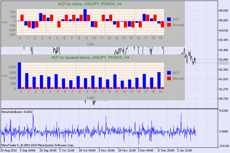
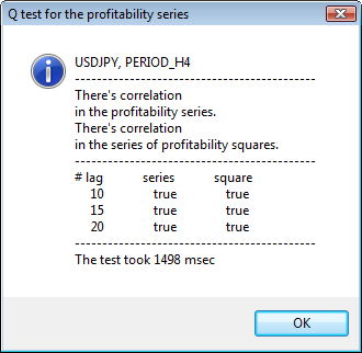
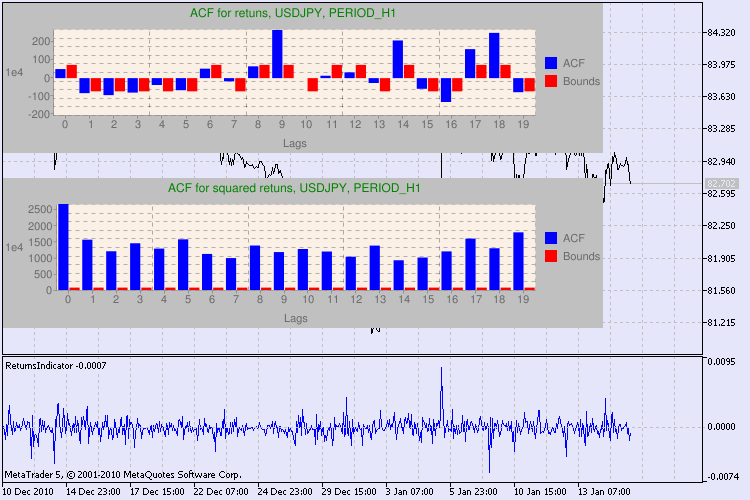
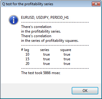
Figure 3. The result of the Q test and the diagram of autocorrelation for USDJPY for different timeframes.

Yes, I searched a lot for a variant of displaying the diagram on a symbol chart in MetaTrader 5. And I have decided that the optimal variant is to use a library of drawing diagrams using Google Chart API, which is described in the corresponding article.

How should we interpret this information? Let's take a look. The upper part of the chart contains the diagram of the autocorrelation function (ACF) for the initial series of returns. At the first diagram we analyze the series of usdjpy of the H4 timeframe. We can see that several values of ACF (blue bars) exceed the limits (red bars). In other words, we see a small autocorrelation in the initial series of returns. The diagram below is the diagram of the autocorrelation function (ACF) of the series of squares of returns of the specified symbol. Everything is clear there, a complete victory of the blue bars. The H1 diagrams are analyzed in the same way.

A few words about the description of the diagram axes. The x axis is clear; it displays the indexes of lags. At the y axis you can see the exponential value, the initial value of ACF is multiplied by. Thus, 1e4 means that the initial value is multiplied by 1e4 (1e4=10000), and 1e2 means multiplying by 100, etc. Such multiplication is done to make the diagram more understandable. 

The upper part of the dialog window displays a symbol or cross pair name and its timeframe. After them, you can see two sentences that tell about the presence or absence of autocorrelation in the initial series of returns and in the series of squares of returns. Then the 10-th, 15-th and 20-th lag are listed as well as the value of autocorrelation in the initial series and in the series of squares. A relative value of autocorrelation is displayed here - a boolean flag during the Q test that determines if there is an autocorrelation at the previous and the specified flags.

In the end, if we see that the autocorrelation exist at the previous and specified flags, then the flag will be equal to true, otherwise - false. In the first case, our series is a "client" for applying the non-linear GARCH model, and in the second case, we need to use simpler analytical models. An attentive reader will note that the initial series of returns of the USDJPY pair slightly correlate with each other, especially the one of the greater timeframe. But the series of squares of returns show autocorrelation.

The time spent on testing is shown in the bottom part of the window.

The entire testing was performed using the GarchTest.mq5 script.

Conclusions

In my article, I described how econometricians analyze time series, or to be more precise, how they start their studies. During it, I had to write many functions and code several types of data (for example, complex numbers). Probably, the visual estimation of an initial series gives nearly the same result as the econometric estimation. However, we agreed to use only precise methods. You know, a good doctor can set a diagnosis without using complex technology and methodology. But anyway, they will study the patient carefully and meticulously.

What do we get from the approach described in the article? Use of the non-linear GARCH models allows representing the analyzed series formally from the mathematical point of view and creating a forecast for a specified number of steps. Further it will help us to simulate the behavior of series at forecast periods and test any ready-made Expert Advisor using the forecasted information.

Location of files:

#	File	Path
1	ReturnsIndicator.mq5	%MetaTrader%\MQL5\Indicators
2	Complex_class.mqh	%MetaTrader%\MQL5\Include
3	FFT_class.mqh	%MetaTrader%\MQL5\Include
4	GarchTest.mq5	%MetaTrader%\MQL5\Scripts

The files and the description of the library google_charts.mqh and Libraries.rar can be downloaded from the previously mentioned article.

Literature used for the article:

1. Analysis of Financial Time Series, Ruey S. Tsay, 2nd Edition, 2005. - 638 pp.
   
2. Applied Econometric Time Series,Walter Enders, John Wiley & Sons, 2nd Edition, 1994. - 448 pp.
   
3. Bollerslev, T., R. F. Engle, and D. B. Nelson. "ARCH Models." Handbook of Econometrics. Vol. 4, Chapter 49, Amsterdam: Elsevier Science B.V.
4. Box, G. E. P., G. M. Jenkins, and G. C. Reinsel. Time Series Analysis: Forecasting and Control. 3rd ed. Upper Saddle River, NJ: Prentice-Hall, 1994.
5. Numerical Recipes in C, The Art of Scientific Computing, 2nd Edition, W.H. Press, B.P. Flannery, S. A. Teukolsky, W. T. Vetterling, 1993. - 1020 pp.
   
6. Gene H. Golub, Charles F. Van Loan. Matrix computations, 1999.
   
7. Porshnev S. V. "Computing mathematics. Series of lectures", S.Pb, 2004.